CPC: learn by identifying the right future
Treat contrastive prediction as a classification problem and inspect what negative sampling assumes.
Representation Learning with Contrastive Predictive Coding · van den Oord, Li & Vinyals · arXiv:1807.03748
Original editorial analysis by Token Lab · Source checked 2026-10-25 · Paper claims and synthetic examples are separated.
Detailed technical articles are available in English and Chinese. This locale shows the English article with localized navigation.
01 · What the paper establishes
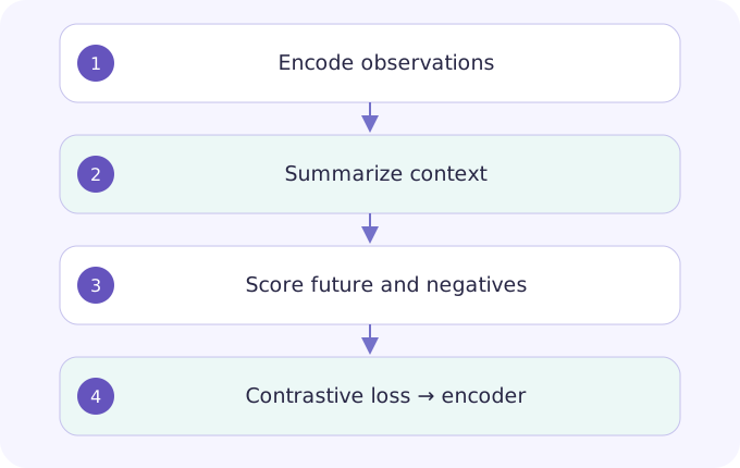
CPC predicts future latent representations from an autoregressive context using a contrastive objective. The paper explores speech, images, text and reinforcement-learning environments. Its mutual-information interpretation depends on the sampling construction and objective assumptions.
Primary source: paper abstract ↗Study guide & lesson outline
LEARNING CONTRACTUnderstand → implement → investigate
Goal: explain the mechanism in this lesson, reproduce one example and test a failure case. Reading alone does not mark mastery.
- Understand: state assumptions, shapes/units and a counterexample.
- Implement: reproduce a numerical example and inspect boundaries.
- Investigate: compare one alternative under a matched budget.
02 · The mechanism
Text / 原始公式
L = −log [exp(s₊/τ) / Σⱼ exp(sⱼ/τ)]
∂L/∂sⱼ = (pⱼ−1[j=+])/τ
Under InfoNCE assumptions: I(X;C) ≥ log N − L_N
The learner does not need to reconstruct every pixel or waveform sample to discriminate a plausible continuation. Context should retain information useful for that discrimination. Negatives define what counts as an alternative; if their distribution is wrong, a shortcut can solve the classification task without the intended representation. N includes the positive candidate in the displayed bound.
Notation and intuition are teaching explanations. Consult the original method for complete assumptions and implementation details.
Mechanism map & worked derivation
| Symbol | Meaning |
|---|---|
| s₊ | Positive candidate compatibility score |
| τ | Temperature, strictly positive |
| N | Total candidates including the positive |
- Rewrite the loss as −s₊/τ+logΣexp(sⱼ/τ). Differentiating the log-sum-exp produces pⱼ/τ; the positive also gets −1/τ.
- For scores [2,1,0,−1] and
, probabilities are approximately [0.643914,0.236883,0.087144,0.032059]. Score gradients are [−0.356086,0.236883,0.087144,0.032059]. - The gradients sum to zero because adding the same constant to every score leaves the distribution unchanged. Use this invariance as a numerical implementation check.
Compare analytical gradients with central differences. Audit whether the negative sampler leaks source identity.
Change one variable. Explain what moves.
Original teaching calculation, not a reproduction of the paper’s benchmark. Bars are relative within this panel; numeric values and units are authoritative.
04 · Work through an example
Original example: four candidates have scores [2,1,0,−1], with the first positive and
05 · Design your experiment
Check analytical score gradients against finite differences. Then deliberately add a false negative and inspect its repulsive gradient. For an encoder POC, split data by source identity before constructing pairs, document the negative sampler and evaluate frozen representations with a held-out probe. Compare downstream metrics, not only contrastive loss.
State one hypothesis; save the configuration and raw results; identify a competing explanation; report the narrowest supported conclusion. Use the linked lab as a local starting point, not a full paper reproduction.
Open related lesson / lab →06 · Limits & reviewer questions
Editorial caution: easier discrimination can mean better shortcuts rather than better semantics. More negatives can introduce false negatives and change optimization. Do not label a toy log-N-minus-loss calculation as a measured information content of a real model.
Why can removing a false negative lower loss without proving better retrieval?
Removing a denominator term makes the classification task easier immediately, even with unchanged embeddings. Retrieval quality requires a separate fixed candidate set and held-out relevance labels.
07 · Read the original
Section 2.3 and Appendix A.1. Write the sampling distribution beside each probability.
Year is the first arXiv submission year. Unversioned links follow revisions; record the exact version in your reproduction report. DeepSeek-R1 here is explicitly pinned to v1.
Continue this topic
SimCLR: augmentation defines what similarity means
Follow two views through a shared encoder and projection head, then audit whether the invariance is valid.
Chen et al. · arXiv:2002.05709