07 · π₀ and continuous action flow matching
Distinguish token prediction, diffusion noise prediction and a continuous velocity field.
Prerequisites: VLA interfaces, differential equations and conditional generation.
Technical posts currently have English and Chinese editions. This locale displays the English article with localized navigation.
Understand the mechanism
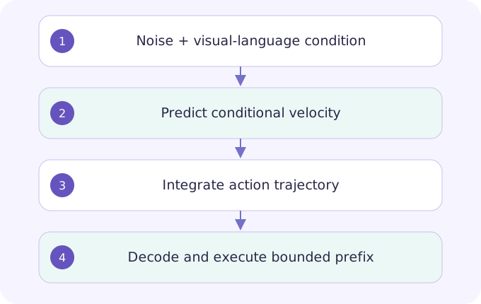
π₀ connects vision-language representations to a flow-based action model. To understand flow matching, begin with a declared interpolation between noise and data and learn its velocity. Time conventions differ across implementations: swapping which endpoint is data changes the target sign. This lesson uses a simple linear path for derivation; it is not a verbatim implementation specification for π₀. Continuous generation still requires numerical integration and a robot-specific action adapter.
Text / 原始公式
x_t = (1−t)ε + t·a,  t ∈ [0,1]
u_t = d x_t/dt = a − ε
L = E[‖vθ(x_t,t,o) − (a−ε)‖²]
x_next = x_t + Δt·vθ(x_t,t,o)
Study guide & lesson outline
LEARNING CONTRACTUnderstand → implement → investigate
Goal: explain the mechanism in this lesson, reproduce one example and test a failure case. Reading alone does not mark mastery.
- Understand: state assumptions, shapes/units and a counterexample.
- Implement: reproduce a numerical example and inspect boundaries.
- Investigate: compare one alternative under a matched budget.
Mechanism map & worked derivation
| Symbol | Meaning |
|---|---|
| ε, a | Noise endpoint and clean action endpoint |
| vθ, t | Learned conditional velocity and interpolation time |
- Take
and At , x_ and the target velocity is 4. - One Euler step of
with the exact velocity reaches at This is a straight-path toy, not a learned-policy result. - For a learned nonlinear field, compare 4, 8 and 16 integration steps under equal initial noise. Record action drift and runtime; more steps do not repair a poorly learned field.
Implement the analytical straight-path example first, including reversed-time tests. Then specify an integration-step ablation for a real model with fixed seeds and deadlines. Keep toy and measured outputs separate.
Original interview exercises & analysis
Answer aloud before revealing the analysis. Add assumptions, a counterexample and a test you would run.
Is flow matching just a single deterministic action?
The field can be deterministic conditional on its input while different initial noise samples produce different actions. Distribution quality still depends on training.
What is a fair comparison with action tokens?
Match data, embodiment, observation history and wall-clock budget; report action precision, success and latency. Different backbone sizes confound a head-only comparison.
Read the primary sources
π₀: A Vision-Language-Action Flow Model ↗ · arXiv PDF ↗
Original Token Lab explanations and synthetic calculations; not measured robot performance. Source links checked 2026-10-25. Unversioned arXiv links may change; record a version for reproduction.