AdamW: where you apply weight decay matters
Separate a loss penalty from parameter shrinkage, then test the difference with an intentionally unequal preconditioner.
Decoupled Weight Decay Regularization · Loshchilov & Hutter · arXiv:1711.05101
Original editorial analysis by Token Lab · Source checked 2026-10-25 · Paper claims and synthetic examples are separated.
01 · What the paper establishes
The paper distinguishes L2 regularization from decoupled weight decay for adaptive optimizers and evaluates the modification on image-classification tasks. It argues that the two operations should not share a name when their updates differ.
Primary source: paper abstract ↗Study guide & lesson outline
LEARNING CONTRACTUnderstand → implement → investigate
Goal: explain the mechanism in this lesson, reproduce one example and test a failure case. Reading alone does not mark mastery.
- Understand: state assumptions, shapes/units and a counterexample.
- Implement: reproduce a numerical example and inspect boundaries.
- Investigate: compare one alternative under a matched budget.
02 · The mechanism
Text / 原始公式
Fixed diagonal preconditioner D:
L2: θ′ = θ − αD(g + λθ)
Decoupled: θ′ = (1−αλ)θ − αDg
Difference in shrinkage: −αλ(D−I)θ
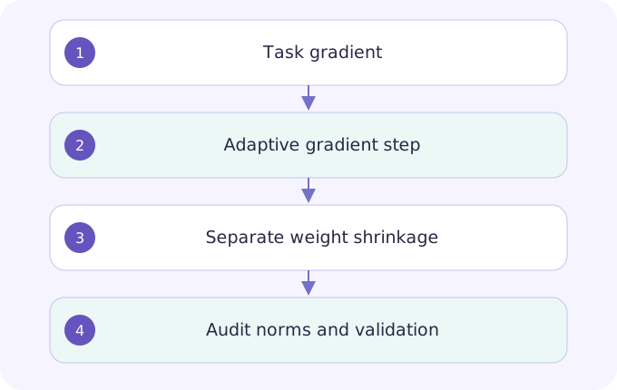
The key question is whether the regularizer passes through the gradient scaling machinery. In the first equation it does; in the second it does not. For plain SGD with
Notation and intuition are teaching explanations. Consult the original method for complete assumptions and implementation details.
Mechanism map & worked derivation
| Symbol | Meaning |
|---|---|
| D | Fixed diagonal scaling for the local comparison |
| λ | Regularization or decay strength; conventions differ |
| Πₜ(1−αλ) | Accumulated decoupled shrinkage without task gradients |
- For a penalty λ||θ||²/2, differentiating gives λθ. Applying a preconditioner to the full gradient also scales this penalty.
- Subtracting the decoupled update from the fixed-D L2 update leaves −αλ(D−I)θ. Equality holds when this expression vanishes, not merely when both options are called weight decay.
- With
and no task gradient, ten decoupled steps retain 0.99¹⁰≈0.904382 of the initial weight. A different step schedule changes this product.
Use a two-coordinate example before a neural model. Then check optimizer source code for decay placement and excluded parameter groups.
Change one variable. Explain what moves.
Original teaching calculation, not a reproduction of the paper’s benchmark. Bars are relative within this panel; numeric values and units are authoritative.
04 · Work through an example
Original example:
05 · Design your experiment
First verify equality for
State one hypothesis; save the configuration and raw results; identify a competing explanation; report the narrowest supported conclusion. Use the linked lab as a local starting point, not a full paper reproduction.
Open related lesson / lab →06 · Limits & reviewer questions
Editorial caution: “decoupled” describes the update mechanism; it does not mean learning rate and decay never interact in an experiment. Accumulated shrinkage depends on the schedule and number of steps. A library option named weight_decay must be checked against its actual optimizer implementation.
Why can equal decay coefficients be an unfair comparison across different training lengths?
With zero task gradients, repeated decoupled updates multiply θ by ∏ₜ(1−αₜλ). Different step counts or schedules change the total shrinkage even when λ is identical.
07 · Read the original
The L2 versus weight-decay comparison and optimizer algorithms; then inspect the tuning experiments.
Year is the first arXiv submission year. Unversioned links follow revisions; record the exact version in your reproduction report. DeepSeek-R1 here is explicitly pinned to v1.
Continue this topic
Adam: understand the update, not just the defaults
Why two moving averages can change the geometry of a training problem. Work through the first step and inspect the effect of bias correction.
Kingma & Ba · arXiv:1412.6980