04 · Demonstrations, behavior cloning and ACT
Design a demonstration dataset and explain why action chunks help without hiding distribution shift.
Prerequisites: Supervised learning, sequence models and control frequency.
Understand the mechanism
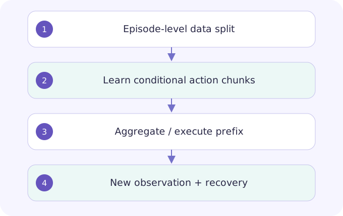
Behavior cloning learns actions from expert observations. At deployment its own mistakes change the observations it sees, creating compounding error. ACT models chunks of future actions and uses a conditional variational formulation; the paper also studies temporal aggregation. These mechanisms do not remove the need for recovery demonstrations. Split data by full episode, operator or scene before normalizing; adjacent frames from one rollout are strongly related.
Text / 原始公式
L_BC = E[‖a − π(o)‖²]
L_CVAE = reconstruction + β·KL(q(z|a,o) ‖ p(z))
āₜ = Σᵢ wᵢ aₜ⁽ⁱ⁾ / Σᵢ wᵢ
Study guide & lesson outline
LEARNING CONTRACTUnderstand → implement → investigate
Goal: explain the mechanism in this lesson, reproduce one example and test a failure case. Reading alone does not mark mastery.
- Understand: state assumptions, shapes/units and a counterexample.
- Implement: reproduce a numerical example and inspect boundaries.
- Investigate: compare one alternative under a matched budget.
Mechanism map & worked derivation
| Symbol | Meaning |
|---|---|
| o, a, z | Observation, action chunk and latent variable |
| wᵢ | Explicitly chosen positive aggregation weights |
- With
at 50 Hz, a chunk spans 0.2 seconds. Executing the entire chunk open-loop delays response to a new disturbance. - Two predictions for the same scalar action are 0.2 and 0.8. With declared weights 0.75 and 0.25, the aggregate is 0.35. State which prediction gets the larger weight.
- If only 2 of 100 episodes include failed grasps, random frame sampling cannot create adequate recovery coverage. Collect or simulate a targeted recovery subset.
Compare single-step BC and chunked prediction on the same demonstrations, compute budget and held-out scenes. Log success, recovery, action smoothness and latency; ablate chunk horizon independently.
Original interview exercises & analysis
Answer aloud before revealing the analysis. Add assumptions, a counterexample and a test you would run.
Why can validation MSE improve while success falls?
MSE averages action errors on expert states. It can obscure contact-critical errors and fails to evaluate the policy-induced state distribution.
What does action chunking trade off?
Temporal coherence and fewer high-level decisions versus stale actions and reduced reactivity. Evaluate execution horizon separately from prediction horizon.
Read the primary sources
ACT / Learning Fine-Grained Bimanual Manipulation ↗ · arXiv PDF ↗
Original Token Lab explanations and synthetic calculations; not measured robot performance. Source links checked 2026-10-25. Unversioned arXiv links may change; record a version for reproduction.