Adam: understand the update, not just the defaults
Why two moving averages can change the geometry of a training problem. Work through the first step and inspect the effect of bias correction.
Adam: A Method for Stochastic Optimization · Kingma & Ba · arXiv:1412.6980
Original editorial analysis by Token Lab · Source checked 2026-10-25 · Paper claims and synthetic examples are separated.
Detailed technical articles are available in English and Chinese. This locale shows the English article with localized navigation.
01 · What the paper establishes
Adam maintains first- and second-moment estimates and corrects their initialization bias. The paper compares optimization behavior on several learning tasks. This is evidence about those experiments, not a guarantee that one optimizer wins everywhere.
Primary source: paper abstract ↗Study guide & lesson outline
LEARNING CONTRACTUnderstand → implement → investigate
Goal: explain the mechanism in this lesson, reproduce one example and test a failure case. Reading alone does not mark mastery.
- Understand: state assumptions, shapes/units and a counterexample.
- Implement: reproduce a numerical example and inspect boundaries.
- Investigate: compare one alternative under a matched budget.
02 · The mechanism
Text / 原始公式
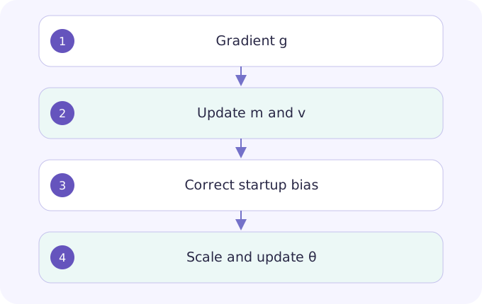
mₜ = β₁mₜ₋₁ + (1−β₁)gₜ
vₜ = β₂vₜ₋₁ + (1−β₂)gₜ²
m̂ₜ = mₜ/(1−β₁ᵗ), v̂ₜ = vₜ/(1−β₂ᵗ)
θₜ = θₜ₋₁ − αm̂ₜ/(√v̂ₜ + ε)
Think of each coordinate as having a direction estimate and a scale estimate. Momentum averages direction; the squared-gradient average supplies the denominator. The denominator is not a Hessian estimate, so calling Adam Newton’s method would be misleading. With zero initialization, early averages are too small; dividing by the missing geometric-series mass corrects that effect under the moment-estimation assumptions.
Notation and intuition are teaching explanations. Consult the original method for complete assumptions and implementation details.
Mechanism map & worked derivation
| Symbol | Meaning |
|---|---|
| gₜ | Current gradient; same shape as parameters |
| mₜ, vₜ | Exponential averages of g and g²; v is not centered variance |
| α, β₁, β₂, ε | Step size, two decay rates and numerical stabilizer |
- Expand the recurrence:
₌₁ᵗβ₁ᵗ⁻ʲgⱼ. If E[gⱼ]=μ is constant, E[mₜ]=(1−β₁ᵗ)μ. This identifies the bias term rather than introducing correction by convention. - Repeat the argument for the raw second moment. Divide by the corresponding geometric mass, then normalize direction by the square root of the corrected second moment.
- For constant
, the second-step uncorrected first- and second-moment estimates are and Correcting yields 2 and 4 again. For a sign-changing gradient, that equality no longer holds: the averages encode history.
Log both raw and corrected moments. If a constant-gradient test does not recover the same moments at every step, inspect indexing and initialization.
Change one variable. Explain what moves.
Original teaching calculation, not a reproduction of the paper’s benchmark. Bars are relative within this panel; numeric values and units are authoritative.
04 · Work through an example
Original worked example: let
05 · Design your experiment
Implement scalar SGD and Adam on
State one hypothesis; save the configuration and raw results; identify a competing explanation; report the narrowest supported conclusion. Use the linked lab as a local starting point, not a full paper reproduction.
Open related lesson / lab →06 · Limits & reviewer questions
Editorial caution: rapid training-loss reduction does not establish better generalization. Compare held-out loss at matched compute and inspect mixed-precision behavior, ε placement and optimizer-state memory. The original convergence discussion should not be read as a universal nonconvex convergence guarantee.
Why can a tiny gradient still produce a noticeable first update?
For nonzero g and negligible ε, bias correction gives g/√g²=sign(g). The learning rate sets the first-step magnitude. Near zero, ε breaks that cancellation; a zero gradient produces zero movement.
07 · Read the original
Algorithm 1 and the bias-correction discussion. Trace the state variables before reading the convergence analysis.
Year is the first arXiv submission year. Unversioned links follow revisions; record the exact version in your reproduction report. DeepSeek-R1 here is explicitly pinned to v1.
Continue this topic
AdamW: where you apply weight decay matters
Separate a loss penalty from parameter shrinkage, then test the difference with an intentionally unequal preconditioner.
Loshchilov & Hutter · arXiv:1711.05101