02 · Perception, state estimation and time
Understand why a sharp image can still produce a stale, uncertain control state.
Prerequisites: Frames, probability and covariance.
Technical posts currently have English and Chinese editions. This locale displays the English article with localized navigation.
Understand the mechanism
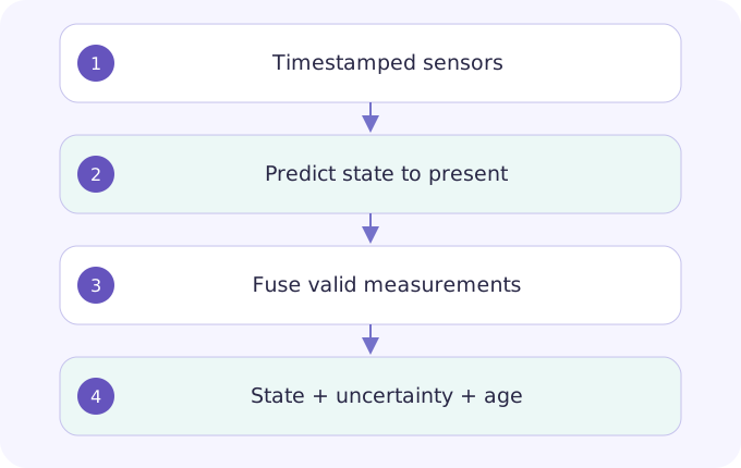
The physical state is partially observed. Cameras, encoders and force sensors have different rates and delays. Keep acquisition time separate from arrival time, and estimate state at the command time. A Kalman-style correction balances predicted uncertainty against measurement uncertainty; correlated errors invalidate a naive independent fusion. Occlusion is missing information, not a zero measurement. Preserve uncertainty and a validity flag through the policy interface.
Text / 原始公式
K = P / (P + R)
x̂_new = x̂_prior + K(z − x̂_prior)
P_new = (1 − K)P
position lag ≈ velocity × sensor age
Study guide & lesson outline
LEARNING CONTRACTUnderstand → implement → investigate
Goal: explain the mechanism in this lesson, reproduce one example and test a failure case. Reading alone does not mark mastery.
- Understand: state assumptions, shapes/units and a counterexample.
- Implement: reproduce a numerical example and inspect boundaries.
- Investigate: compare one alternative under a matched budget.
Mechanism map & worked derivation
| Symbol | Meaning |
|---|---|
| P, R | Scalar prior and measurement variances |
| z, K | Measurement and Kalman gain |
- Prior position is 1.0 m with
m²; sensor reports 1.2 m with m². - The corrected position is 1.16 m and variance 0.008 m². This scalar example assumes unbiased independent Gaussian noise.
- At 0.5 m/s, an 80 ms old observation is displaced by approximately 4 cm under constant velocity. Better classification accuracy cannot remove this lag.
Create a synthetic constant-velocity trace with seeded noise, dropped frames and delay. Compare raw versus filtered RMSE and lag. Hold out the delay pattern, not random adjacent frames.
Original interview exercises & analysis
Answer aloud before revealing the analysis. Add assumptions, a counterexample and a test you would run.
Why can fusion be overconfident?
Two estimates may share the same camera or calibration error. Treating them as independent double-counts evidence; track correlation or conservatively fuse.
What should happen during occlusion?
Predict with growing uncertainty and apply an age/uncertainty gate. Define when to pause or request a new view; do not invent observations.
Read the primary sources
Underactuated Robotics — Russ Tedrake ↗
Original Token Lab explanations and synthetic calculations; not measured robot performance. Source links checked 2026-10-25. Unversioned arXiv links may change; record a version for reproduction.