From bytes to a trained Transformer: build a language model from scratch
A complete CPU-sized project: byte encoding, causal attention, loss, AdamW, checkpoints and generation—with runnable Python and explicit limits.
Sources & version details
In this article
1. What we are building—and what a language model learns
Imagine an operations console that completes “node 107: status is”. We will construct a causal Transformer, initialize every weight randomly, train it on an original synthetic corpus, save a checkpoint and generate bytes. No pretrained weights, downloaded dataset or model API is needed. The complete program uses PyTorch for tensors, automatic differentiation and optimizer primitives; “from scratch” means implementing the architecture and training pipeline, not writing GPU kernels or an autodiff engine.
The complete learning and generation pipeline
Scroll horizontally on small screens, or open the full-size diagram. View full-size diagram
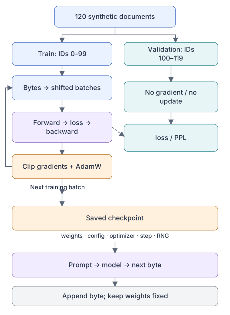
A language model estimates the next-token distribution conditioned on previous tokens. Its learned weights encode statistical regularities, not a database of verified propositions. Our 134,912-parameter model is deliberately small enough for a CPU. It teaches the computational skeleton of a larger model, but it is neither a general assistant nor an instruction-following model. The running example will expose this distinction: learning the syntax of status messages does not guarantee learning which node should be busy.
You should be able to multiply a matrix by a vector, interpret a probability distribution and apply the chain rule. Matrix multiplication mixes features; softmax converts scores to probabilities; the chain rule sends the loss signal through every layer. If these operations are unfamiliar, use the foundation tutorials collected at the end before attempting to change the model.
2. Prepare the environment and project files
Download the complete project below and extract it into a new directory. tiny_lm.py contains the model, synthetic corpus, training loop and built-in checks; generate.py is the separate inference entry point. Keep the files beside one another. You can use the downloaded implementation as a reference while reconstructing each function in the following chapters. The excerpts are real portions of that implementation, not independent programs to concatenate blindly.
The recorded reference environment is Linux, Python 3.12 and PyTorch 2.5.1 CPU. Create an isolated virtual environment and install the pinned CPU package using the commands below. Installation downloads software; training itself uses an original built-in corpus and makes no model API calls. A GPU is not required. Other platforms may need a compatible official PyTorch wheel and can produce slightly different numerical results.
The project produces tiny.pt, a checkpoint containing configuration, model weights, optimizer state, step and random-generator state. The tutorial first explains how to construct that artifact, then how to load it in another process. Run the training, verification and generation commands together in the final practice section after completing the component walkthrough. No checkpoint or pretrained model is required at the start.
Download the complete project ZIP
unzip from-zero-lm.zip -d tokenlab-lm
cd tokenlab-lm
python3.12 -m venv .venv
. .venv/bin/activate
python -m pip install torch==2.5.1 --index-url https://download.pytorch.org/whl/cpu
3. From documents to supervised pairs
The built-in corpus contains 120 status documents. Even IDs are ready and odd IDs busy. We split IDs 0–99 into training and 100–119 into validation before forming windows. Each document ends with a newline. This prevents windows from the same document being randomly scattered across both sets; it does not make the synthetic validation distribution independent of the training template. Both share the same grammar, so the result measures interpolation within a tiny distribution.
UTF-8 bytes give a fixed vocabulary
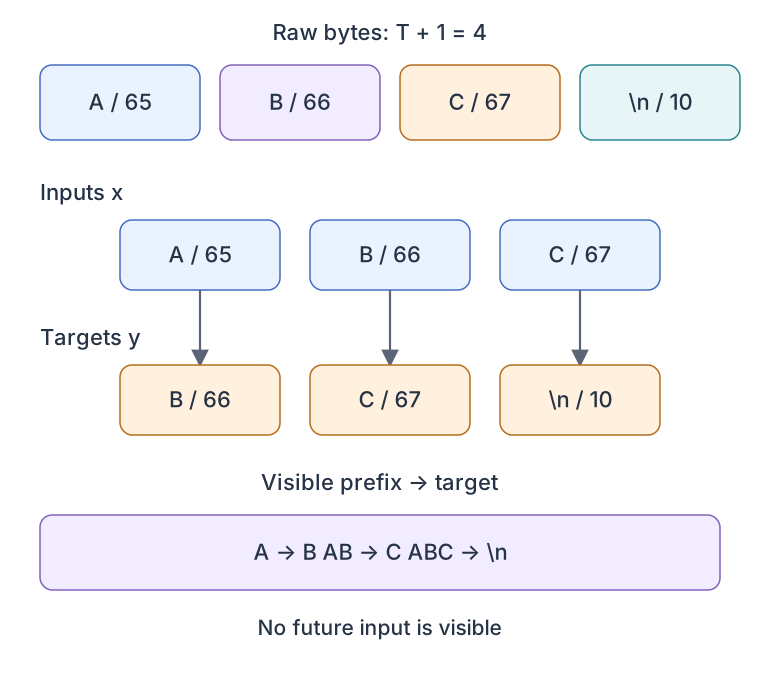
For each sampled start position take T+1 bytes. The first T are inputs and the last T targets. With [65,66,67,10], input [65,66,67] predicts [66,67,10]. A batch has shape [B,T], not [B,T,V]. Concatenating documents permits windows across newlines; use explicit document boundaries and loss masks if cross-document prediction is inappropriate.
Implement the data contract
Write corpus() and batch() in tiny_lm.py before wiring the training loop. corpus() returns two byte strings; batch() converts only the selected split into torch.long token IDs. A sampled start must leave room for T+1 bytes: with N bytes there are N−T valid starts, numbered 0 through N−T−1. Each sample returns two length-32 rows. With 16 samples, both x and y are [16,32]. The same generator object is reused so its state advances between steps rather than repeating one batch.
Implementation excerpt · use the complete project for execution
def corpus():
    # Original synthetic sentences. Split document IDs BEFORE window extraction.
    docs = [f'node {i:03d}: status is {"ready" if i % 2 == 0 else "busy"}.\n' for i in range(120)]
    return ''.join(docs[:100]).encode(), ''.join(docs[100:]).encode()

def batch(raw, generator, size=16):
    data=torch.tensor(list(raw), dtype=torch.long)
    t=CFG['context']
    starts=torch.randint(len(data)-t, (size,), generator=generator)
    return torch.stack([data[i:i+t] for i in starts]), torch.stack([data[i+1:i+t+1] for i in starts])
The split is a statistical boundary, not merely a filename choice. If you change to --text, prepare the corpus before invoking the script; each split must contain more than 32 bytes. The program concatenates documents and samples byte windows, so it does not provide document-level masking or deduplication. Keep this behavior explicit when interpreting its loss: a larger corpus changes both the data distribution and how often a passage is sampled.
How one sequence becomes three prediction targets
Scroll horizontally on small screens, or open the full-size diagram. View full-size diagram
4. Attention is a weighted read, with a causal boundary
The implementation uses
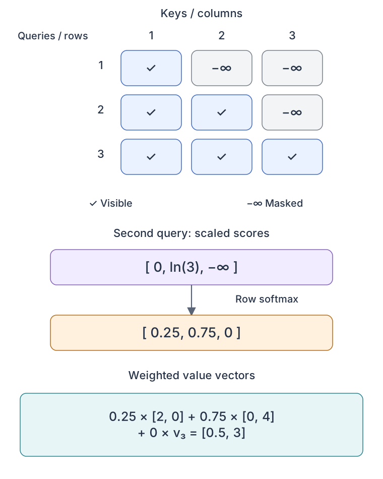
Mask entries with key position j greater than query position i to negative infinity before softmax. Apply softmax over keys, then multiply by V. For a two-key teaching example with scaled logits [0,log 3], probabilities are [0.25,0.75]. Values [2,0] and [0,4] yield [0.5,3]. At the first position the second key is masked, so the result is [2,0]. The actual implementation uses stable PyTorch softmax; never normalize along the batch axis.
Merge four [T,16] heads into [T,64] and apply an output projection. The score tensor holds 16×4×32×32=65,536 float32 values: 256 KiB per layer for scores alone. Dense attention scales quadratically in T; the full block also pays for feature projections. Our clear implementation is not FlashAttention, and it does not use KV caching. A visible attention weight is a mixing coefficient, not proof of a causal explanation of the model’s decision.
Trace the head split and merge
The QKV projection changes [16,32,64] into [16,32,192], then chunk returns three tensors of width 64. Reshape each into [16,32,4,16] and transpose time and heads to obtain [16,4,32,16]. The score product is now [16,4,32,32]; its last axis indexes keys, so softmax(dim=-1) normalizes over candidate source positions for each query. The lower-triangular buffer broadcasts over batch and heads. It is saved in the state but is not an optimizer parameter.
Implementation excerpt · use the complete project for execution
class Attention(nn.Module):
    def __init__(self, width, heads, context):
        super().__init__()
        assert width % heads == 0
        self.heads, self.dim = heads, width // heads
        self.qkv = nn.Linear(width, 3 * width)
        self.out = nn.Linear(width, width)
        self.register_buffer('mask', torch.ones(context, context, dtype=torch.bool).tril())

    def forward(self, x):
        b, t, c = x.shape
        q, k, v = self.qkv(x).chunk(3, dim=-1)
        q, k, v = [a.view(b, t, self.heads, self.dim).transpose(1, 2) for a in (q, k, v)]
        scores = q @ k.transpose(-2, -1) / math.sqrt(self.dim)
        scores = scores.masked_fill(~self.mask[:t, :t], float('-inf'))
        mixed = scores.softmax(dim=-1) @ v
        return self.out(mixed.transpose(1, 2).contiguous().view(b, t, c))
After weighted aggregation, the result is [16,4,32,16]. Transpose back, make the storage contiguous, and merge the four heads into width 64 before the output projection. Omitting that transpose would mix time with head features. The scale is √16=4 for each head, not √64=8 for the whole model. Masking after softmax without renormalization would lose probability mass; this implementation masks scores before normalization.
Causal attention: from a mask to a weighted vector
Scroll horizontally on small screens, or open the full-size diagram. View full-size diagram
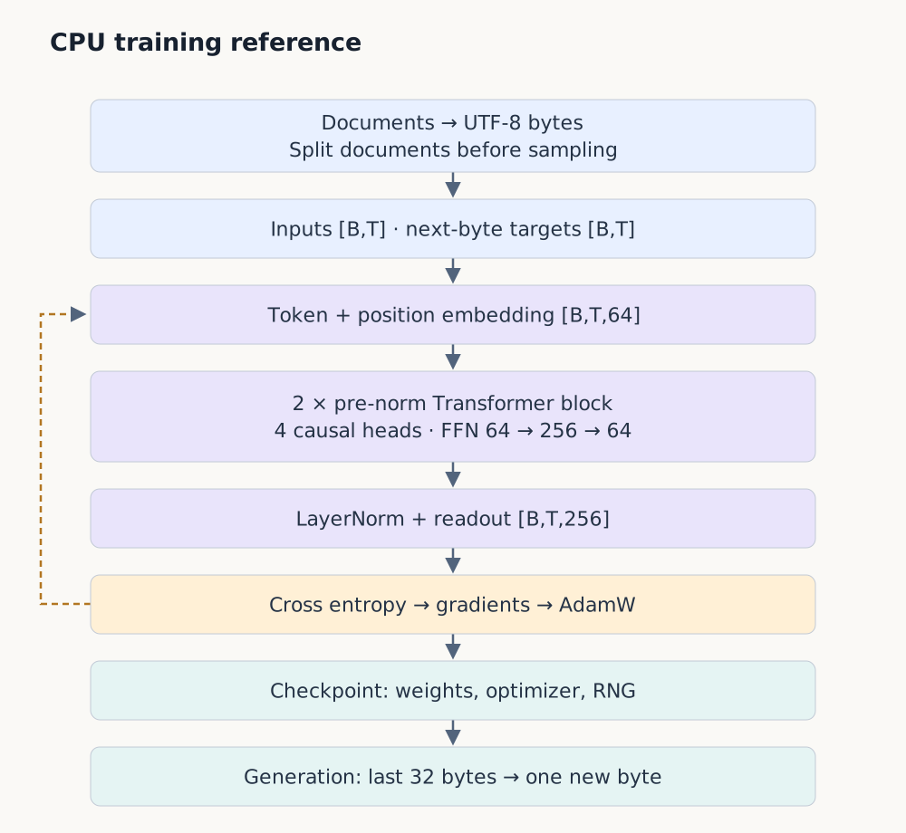
5. Trace every tensor through the decoder
Use
Each pre-normalized block has two residual updates: attention on LayerNorm(X), then a two-layer feed-forward network on the normalized new state. The feed-forward network expands 64→256, applies GELU and projects 256→64 independently at each position. Attention mixes positions; the feed-forward part transforms features. Residual additions preserve a direct route through depth, but they do not eliminate all optimization problems.
After two blocks, a final LayerNorm and a separate [64,256] projection produce logits [16,32,256]. We deliberately do not tie the output weights to token embeddings. Including biases and normalization parameters yields exactly 134,912 trainable parameters. At float32 the parameters alone occupy 539,648 bytes; gradients, Adam moments and saved activations add more. Do not quote this number as total training memory.
LayerNorm computes a separate mean and variance across the D features of each token, then applies learned scale and bias. It does not mix examples or look ahead in time. GELU is a smooth nonlinear gate; without nonlinearities, stacked position-wise linear maps collapse to a single linear map. In the block equation, use a column vector for each token: W₁ is [4D,D] and W₂ is [D,4D]. The batched Python Linear operation stores these weights in that orientation and multiplies input rows by their transpose.
Assemble the decoder in dependency order
Implement Attention first, then Block, then TinyLM. nn.Module registers child layers so model.parameters() reaches every trainable weight and state_dict() can serialize them. Token IDs index embedding rows; they are not multiplied as numerical magnitudes. Position embeddings distinguish identical bytes occurring at different positions. Each residual branch must return the same [B,T,D] shape as its input, because addition is elementwise. Two blocks transform contextual features; the final linear head maps 64 features to 256 unnormalized class scores.
Implementation excerpt · use the complete project for execution
class Block(nn.Module):
    def __init__(self, c):
        super().__init__()
        d=c['width']
        self.n1, self.n2 = nn.LayerNorm(d), nn.LayerNorm(d)
        self.attn = Attention(d, c['heads'], c['context'])
        self.ff = nn.Sequential(nn.Linear(d, 4*d), nn.GELU(), nn.Linear(4*d, d))

    def forward(self, x):
        x = x + self.attn(self.n1(x))
        return x + self.ff(self.n2(x))

class TinyLM(nn.Module):
    def __init__(self, cfg=CFG):
        super().__init__()
        self.cfg = cfg
        self.tokens = nn.Embedding(cfg['vocab'], cfg['width'])
        self.positions = nn.Embedding(cfg['context'], cfg['width'])
        self.blocks = nn.Sequential(*[Block(cfg) for _ in range(cfg['layers'])])
        self.norm = nn.LayerNorm(cfg['width'])
        self.head = nn.Linear(cfg['width'], cfg['vocab'], bias=False)
        self.apply(self.init)

    @staticmethod
    def init(m):
        if isinstance(m, (nn.Linear, nn.Embedding)):
            nn.init.normal_(m.weight, std=.02)
            if getattr(m, 'bias', None) is not None: nn.init.zeros_(m.bias)

    def forward(self, ids):
        if ids.ndim != 2 or not 0 < ids.shape[1] <= self.cfg['context']:
            raise ValueError('Expected [batch, time], 1 <= time <= context')
        x = self.tokens(ids) + self.positions(torch.arange(ids.shape[1], device=ids.device))
        return self.head(self.norm(self.blocks(x)))
Keep CFG as the single architecture definition when constructing and reloading the model. Changing width, vocabulary or layer count changes parameter shapes; an old checkpoint cannot generally load into the new architecture. The forward method intentionally rejects sequences longer than 32 instead of silently indexing beyond the position table. Wider context requires changing that table and the mask as well as reconsidering quadratic attention memory; it is not just a command-line input limit.
| Stage | Input → output | Boundary |
|---|---|---|
| Embedding | [B,T] → [B,T,D] | |
| Q / K / V | [B,T,D] → [B,H,T,D/H] | 64 ÷ 4 = 16 |
| Attention | [B,H,T,T] × [B,H,T,D/H] | j≤i |
| Readout | [B,T,D] → [B,T,V] | 134,912 parameters |
| Loss | [BT,V] + [BT] → scalar | nats / byte |
6. Loss, gradients and the update loop
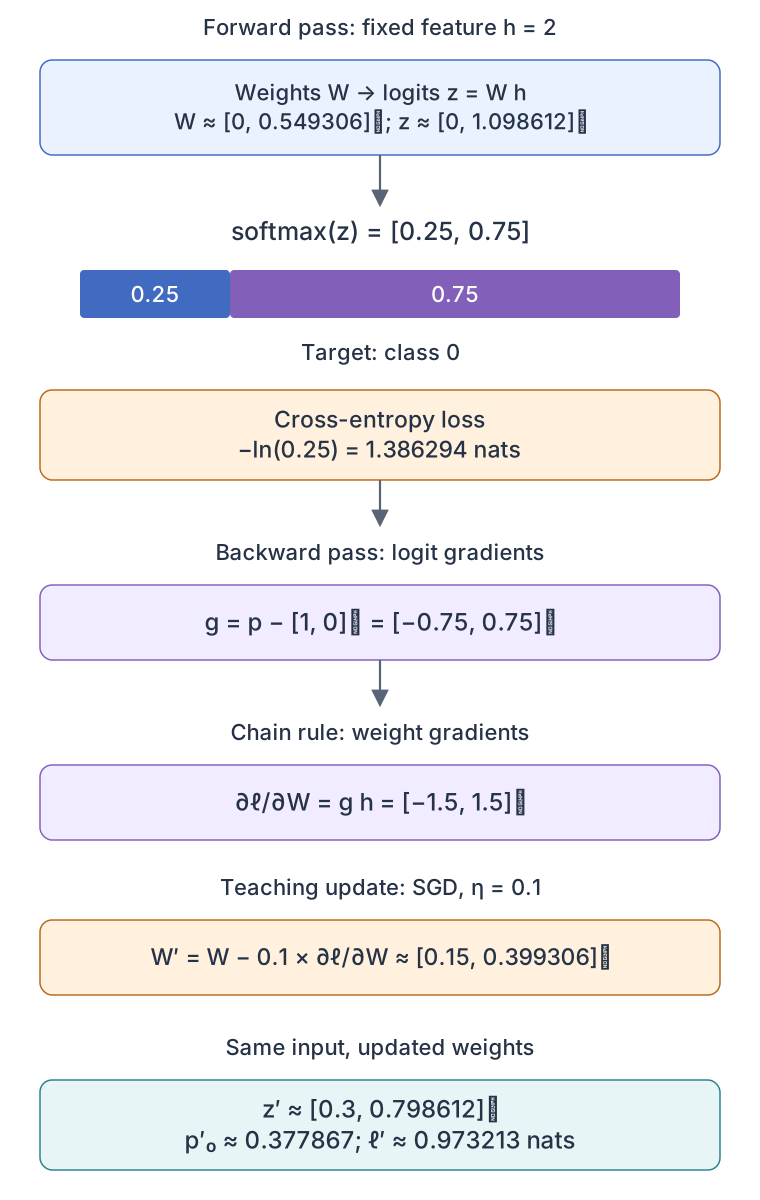
Training performs teacher forcing: every position sees the real preceding bytes, not previously sampled predictions. Flatten logits [B,T,V] into [BT,V] and targets into [BT], then pass raw logits to cross_entropy. It combines log-softmax and negative log likelihood stably. Do not apply softmax beforehand. If the correct next byte receives probability 0.25, its loss is −
Autograd computes derivatives through embeddings, attention and feed-forward layers. Each step clears old gradients, computes loss, backpropagates, clips the total gradient norm to 1, then applies AdamW. Its first and second gradient moments adapt update scale; decoupled weight decay shrinks parameters separately. The teaching script applies decay uniformly, including normalization parameters; production recipes often exclude biases and normalization, which must be documented as an experimental choice.
The nominal peak learning rate is 0.002, with 20 warmup steps multiplied by a cosine factor that approaches 10% at the end. A learning rate is an update multiplier, not a probability of learning. Too large can destabilize training; too small can leave a flat-looking curve. Saving optimizer moments, model configuration, step and random-generator states makes a resumable checkpoint possible. This script verifies reload but does not implement a resume command: a true resume must also restore schedule position and data order.
For one target class y and logits z, the cross-entropy derivative is pᵢ−1[
To connect the scalar loss to actual parameters, isolate the output layer. Let h be one normalized hidden column vector of shape [D,1], W the stored output weight matrix [V,D], and
Implement one optimization step, then repeat
For each step, obtain a fresh x,y batch, set the learning rate, and clear gradients. loss() flattens 16×32 positions into 512 classification examples, each with 256 possible byte classes. backward() accumulates gradients in parameter.grad; opt.step() uses them to update the weights, so clearing old gradients is necessary unless accumulation is intentional. The 300-step run processes 153,600 sampled target positions, with repeats; that is not the count of distinct corpus bytes or training epochs.
Implementation excerpt · use the complete project for execution
def loss(model, x, y):
    logits=model(x)
return F.cross_entropy(logits.reshape(-1, CFG['vocab']), y.reshape(-1))opt=torch.optim.AdamW(model.parameters(),lr=.002,weight_decay=.01)
before=heldout_loss(model,val)
for step in range(args.steps):
model.train();x,y=batch(train,generator)
lr=.002*min((step+1)/20,1)*(.1+.9*.5*(1+math.cos(math.pi*step/args.steps)))
for group in opt.param_groups:group['lr']=lr
opt.zero_grad(set_to_none=True);value=loss(model,x,y)
if not torch.isfinite(value):raise RuntimeError('nonfinite loss')
value.backward();nn.utils.clip_grad_norm_(model.parameters(),1.0);opt.step()The scheduler multiplies a warmup factor by a cosine factor; the cosine already progresses during warmup, so the actual maximum is slightly below the nominal 0.002. After training, save parameters and the optimizer separately inside the checkpoint dictionary. Gradients themselves are not the trained model. The saved optimizer and random states support future resume work, but this project reloads only model weights for generation and does not implement uninterrupted-training equivalence.
From prediction error to a weight update
Scroll horizontally on small screens, or open the full-size diagram. View full-size diagram
7. From a checkpoint to generated text
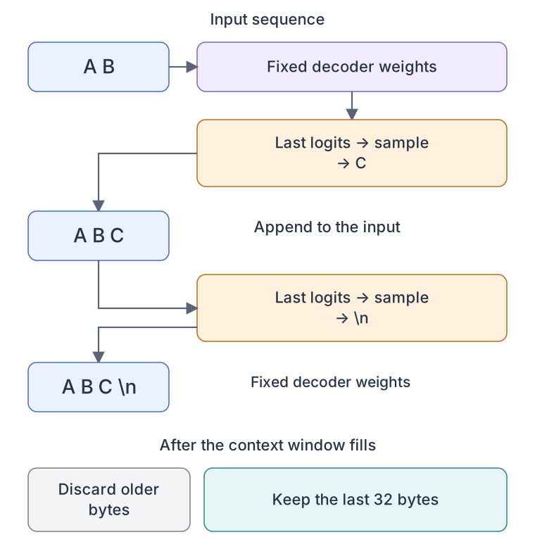
Inference encodes a nonempty prompt, selects its last 32 bytes, runs the decoder and takes only the final position’s logits. Divide them by a positive temperature, keep the top k logits, normalize and sample one byte. Append it and repeat. Temperature below one sharpens probabilities; top-k removes the tail before renormalization. Neither improves factual reliability by itself. Generation here stops after a fixed number of bytes, not an EOS token.
Cropping resets learned positions to 0…31 each iteration and forgets older content. Recomputing the whole window makes the code easy to inspect but expensive for long outputs. A real KV cache stores earlier keys and values instead; it requires careful positional semantics, invalidation and equivalence checks. Do not simply append cached vectors while resetting learned positions and expect identical outputs.
UTF-8 decoding uses replacement for incomplete byte sequences, so arbitrary generations may contain replacement characters. The fixture is ASCII and avoids most of this issue. To become a useful assistant, a model additionally needs much broader lawful data, sufficient capacity, instruction training, deployment infrastructure and an evidence-based safety process. Scaling parameters alone cannot provide these properties. This tutorial’s model is also not strong enough to drive the companion Agent: that project supplies a separate adapter for a capable local instruction model.
Load the checkpoint in a separate process
Create generate.py beside tiny_lm.py so it can import TinyLM without triggering training; the main guard prevents that side effect. Load the checkpoint onto CPU, reconstruct the architecture from its saved config, then load its model state and switch to eval mode. Reset the sampling seed after construction because parameter initialization itself consumes random numbers. This separates training artifacts from an inference entry point and makes repeated runs with the same environment and seed comparable.
Implementation excerpt · use the complete project for execution
"""Generate from a trusted checkpoint without retraining."""
import argparse,torch
from tiny_lm import TinyLM
p=argparse.ArgumentParser();p.add_argument('checkpoint');p.add_argument('--prompt',default='node 10');p.add_argument('--seed',type=int,default=42)
a=p.parse_args();torch.set_num_threads(1);torch.manual_seed(a.seed)
s=torch.load(a.checkpoint,map_location='cpu',weights_only=True)
m=TinyLM(s['config']);m.load_state_dict(s['model']);m.eval()
torch.manual_seed(a.seed)
print(m.generate(a.prompt))
Call python generate.py tiny.pt --prompt "node 10" after the training command completes. The returned text includes the original prompt plus 80 generated bytes. It is a command-line model, not an HTTP API, and it has neither instruction tuning nor an Agent protocol. A useful next extension is a separate inference service with input limits and queueing, but do not label that service implemented until it exists. Use only trusted checkpoints; weights_only reduces loader exposure but does not establish file provenance.
Autoregressive generation, one byte at a time
Scroll horizontally on small screens, or open the full-size diagram. View full-size diagram
8. Practice, verification and interview exercises
Run the complete program below. It checks output shapes, future-token non-interference, context bounds, one readout derivative by central finite differences, and exact checkpoint logits. For a fair extension, hold corpus, split, seeds, steps and validation protocol fixed: compare a bigram baseline, one versus two blocks, and the trained model versus random initialization. Report held-out loss and parity-rule accuracy separately; repeat over at least three seeds. Removing the causal mask is a deliberately invalid leakage demonstration, never a legitimate competing model. For your own text, inspect licensing and split before --text, and do not reuse validation for model selection indefinitely.
Complete implementation and commands
Download the complete project ZIP
python tiny_lm.py --steps 300 --output tiny.pt
python generate.py tiny.pt --prompt 'node 10'
# Optional: your own licensed UTF-8 text, after data preparation
# python tiny_lm.py --text corpus.txt --steps 300 --output own.pttiny_lm.py
"""Original Token Lab byte-level causal LM. Python 3.12 / torch 2.5.1 CPU.
Run: python tiny_lm.py --steps 300 --output tiny.pt
No pretrained weights, downloads, model API or third-party dataset.
"""
import argparse
import math
from pathlib import Path
import torch
from torch import nn
from torch.nn import functional as F
CFG = dict(vocab=256, context=32, width=64, heads=4, layers=2)
class Attention(nn.Module):
def __init__(self, width, heads, context):
super().__init__()
assert width % heads == 0
self.heads, self.dim = heads, width // heads
self.qkv = nn.Linear(width, 3 * width)
self.out = nn.Linear(width, width)
self.register_buffer('mask', torch.ones(context, context, dtype=torch.bool).tril())
def forward(self, x):
b, t, c = x.shape
q, k, v = self.qkv(x).chunk(3, dim=-1)
q, k, v = [a.view(b, t, self.heads, self.dim).transpose(1, 2) for a in (q, k, v)]
scores = q @ k.transpose(-2, -1) / math.sqrt(self.dim)
scores = scores.masked_fill(~self.mask[:t, :t], float('-inf'))
mixed = scores.softmax(dim=-1) @ v
return self.out(mixed.transpose(1, 2).contiguous().view(b, t, c))
class Block(nn.Module):
def __init__(self, c):
super().__init__()
d=c['width']
self.n1, self.n2 = nn.LayerNorm(d), nn.LayerNorm(d)
self.attn = Attention(d, c['heads'], c['context'])
self.ff = nn.Sequential(nn.Linear(d, 4*d), nn.GELU(), nn.Linear(4*d, d))
def forward(self, x):
x = x + self.attn(self.n1(x))
return x + self.ff(self.n2(x))
class TinyLM(nn.Module):
def __init__(self, cfg=CFG):
super().__init__()
self.cfg = cfg
self.tokens = nn.Embedding(cfg['vocab'], cfg['width'])
self.positions = nn.Embedding(cfg['context'], cfg['width'])
self.blocks = nn.Sequential(*[Block(cfg) for _ in range(cfg['layers'])])
self.norm = nn.LayerNorm(cfg['width'])
self.head = nn.Linear(cfg['width'], cfg['vocab'], bias=False)
self.apply(self.init)
@staticmethod
def init(m):
if isinstance(m, (nn.Linear, nn.Embedding)):
nn.init.normal_(m.weight, std=.02)
if getattr(m, 'bias', None) is not None: nn.init.zeros_(m.bias)
def forward(self, ids):
if ids.ndim != 2 or not 0 < ids.shape[1] <= self.cfg['context']:
raise ValueError('Expected [batch, time], 1 <= time <= context')
x = self.tokens(ids) + self.positions(torch.arange(ids.shape[1], device=ids.device))
return self.head(self.norm(self.blocks(x)))
@torch.no_grad()
def generate(self, prompt, count=80, temperature=.8, top_k=20):
if not prompt or temperature <= 0 or not 1 <= top_k <= self.cfg['vocab']:
raise ValueError('Nonempty prompt, positive temperature, valid top_k required')
self.eval()
ids = torch.tensor([list(prompt.encode('utf-8'))], dtype=torch.long)
for _ in range(count):
logits = self(ids[:, -self.cfg['context']:])[:, -1, :] / temperature
threshold = logits.topk(top_k).values[:, -1:]
logits = logits.masked_fill(logits < threshold, float('-inf'))
ids = torch.cat((ids, torch.multinomial(logits.softmax(-1), 1)), dim=1)
return bytes(ids[0].tolist()).decode('utf-8', errors='replace')
def corpus():
# Original synthetic sentences. Split document IDs BEFORE window extraction.
docs = [f'node {i:03d}: status is {"ready" if i % 2 == 0 else "busy"}.\n' for i in range(120)]
return ''.join(docs[:100]).encode(), ''.join(docs[100:]).encode()
def batch(raw, generator, size=16):
data=torch.tensor(list(raw), dtype=torch.long)
t=CFG['context']
starts=torch.randint(len(data)-t, (size,), generator=generator)
return torch.stack([data[i:i+t] for i in starts]), torch.stack([data[i+1:i+t+1] for i in starts])
def loss(model, x, y):
logits=model(x)
return F.cross_entropy(logits.reshape(-1, CFG['vocab']), y.reshape(-1))
@torch.no_grad()
def heldout_loss(model, raw):
model.eval()
data=torch.tensor(list(raw),dtype=torch.long)
total, count=0.,0
for i in range(0,len(data)-1,CFG['context']):
t=min(CFG['context'],len(data)-1-i)
x,y=data[i:i+t][None,:],data[i+1:i+t+1][None,:]
total += loss(model,x,y).item()*t
count += t
return total/count
def checks(model):
model.eval()
x=torch.arange(12)[None,:]
changed=x.clone();changed[:,7:]=200
with torch.no_grad():
a,b=model(x),model(changed)
assert a.shape == (1,12,256)
assert torch.allclose(a[:,:7],b[:,:7],atol=1e-6), 'future leak'
try:model(torch.zeros(1,33,dtype=torch.long))
except ValueError:pass
else:raise AssertionError('context overflow accepted')
# One coordinate of the readout gradient, central finite difference.
target=torch.arange(1,13)[None,:]
model.zero_grad(set_to_none=True)
loss(model,x,target).backward()
analytical=model.head.weight.grad[1,0].item()
original=model.head.weight[1,0].item();eps=.01
with torch.no_grad():
model.head.weight[1,0]=original+eps;plus=loss(model,x,target).item()
model.head.weight[1,0]=original-eps;minus=loss(model,x,target).item()
model.head.weight[1,0]=original
assert abs(analytical-(plus-minus)/(2*eps))<.002, 'gradient mismatch'
def main():
p=argparse.ArgumentParser();p.add_argument('--steps',type=int,default=300)
p.add_argument('--output',default='tiny.pt');p.add_argument('--text',help='Optional owned UTF-8 corpus; chronological 90/10 split')
args=p.parse_args()
if args.steps<1:raise ValueError('steps must be positive')
torch.set_num_threads(1);torch.manual_seed(42);torch.use_deterministic_algorithms(True)
generator=torch.Generator().manual_seed(123)
train,val=corpus()
if args.text:
raw=Path(args.text).read_text(encoding='utf-8').encode();cut=int(.9*len(raw));train,val=raw[:cut],raw[cut:]
if min(len(train),len(val))<=CFG['context']:raise ValueError('each split must exceed context')
model=TinyLM();checks(model)
opt=torch.optim.AdamW(model.parameters(),lr=.002,weight_decay=.01)
    before=heldout_loss(model,val)
    for step in range(args.steps):
        model.train();x,y=batch(train,generator)
        lr=.002*min((step+1)/20,1)*(.1+.9*.5*(1+math.cos(math.pi*step/args.steps)))
        for group in opt.param_groups:group['lr']=lr
        opt.zero_grad(set_to_none=True);value=loss(model,x,y)
        if not torch.isfinite(value):raise RuntimeError('nonfinite loss')
        value.backward();nn.utils.clip_grad_norm_(model.parameters(),1.0);opt.step()
after=heldout_loss(model,val)
torch.save({'config':CFG,'model':model.state_dict(),'optimizer':opt.state_dict(),
'step':args.steps,'rng':torch.get_rng_state(),'batch_rng':generator.get_state()},args.output)
saved=torch.load(args.output,weights_only=True);restored=TinyLM(saved['config']);restored.load_state_dict(saved['model']);restored.eval();model.eval()
probe=torch.tensor([[1,2,3]])
assert torch.equal(model(probe),restored(probe)), 'checkpoint mismatch'
checks(model)
print(f'parameters={sum(p.numel() for p in model.parameters())}')
print(f'validation_nats_per_byte: {before:.6f} -> {after:.6f}')
print(f'validation_perplexity_per_byte={math.exp(after):.6f}')
print('checks: shapes, causal mask, context bound, gradient, checkpoint passed')
if not args.text and args.steps>=300:assert after<before, 'synthetic learning failed'
torch.manual_seed(42);print('sample='+repr(model.generate('node 10')))
if __name__=='__main__':main()
generate.py
"""Generate from a trusted checkpoint without retraining."""
import argparse,torch
from tiny_lm import TinyLM
p=argparse.ArgumentParser();p.add_argument('checkpoint');p.add_argument('--prompt',default='node 10');p.add_argument('--seed',type=int,default=42)
a=p.parse_args();torch.set_num_threads(1);torch.manual_seed(a.seed)
s=torch.load(a.checkpoint,map_location='cpu',weights_only=True)
m=TinyLM(s['config']);m.load_state_dict(s['model']);m.eval()
torch.manual_seed(a.seed)
print(m.generate(a.prompt))
Observed output and verification limits
Locally executed with Python 3.12 and PyTorch 2.5.1+cpu, one CPU thread, initialization seed 42 and batch seed 123, 300 optimizer steps. Held-out loss fell from 5.575623 to 0.546086 nats/byte; byte perplexity was 1.726483. These are measurements on the synthetic status corpus, not a benchmark on natural language. The generated node 046 is busy even though the data rule makes even nodes ready: low average loss does not establish rule learning. The validation protocol resets context every 32-byte block and weights loss by token count. Small numeric differences across platforms are possible.
parameters=134912
validation_nats_per_byte: 5.575623 -> 0.546086
validation_perplexity_per_byte=1.726483
checks: shapes, causal mask, context bound, gradient, checkpoint passed
sample='node 107: status is busy.\nnode 046: status is busy.\nnode 096: status is ready.\nnode 081'
Troubleshooting after the first run
| Symptom | Meaning | Next action |
|---|---|---|
| ModuleNotFoundError: torch | The running Python cannot see the installed dependency. | Activate .venv; compare python -m pip --version and python -c "import sys; print(sys.executable)". Install through that same interpreter. |
| Checkpoint missing or incompatible | Training did not finish, the path is wrong, or configuration changed. | Use the path passed to --output. Load the saved config before state_dict; do not suppress shape errors. Retrain after intentional architecture changes. |
| Low loss, incorrect node status | Byte prediction quality is not task-rule accuracy. | Compare generated even/odd status labels with the corpus rule; report rule accuracy separately. Keep training settings and prompts fixed for a fair comparison. |
Original interview practice—not company interview reports
Score each answer 1–5: 1 names a term; 2 defines it correctly; 3 traces the concrete example; 4 explains a failure and its mitigation; 5 proposes a fair comparison and states what the evidence cannot establish. Code without an explanation is not a full-score answer.
1. Why can a model appear excellent after removing the causal mask?
Hint
Locate the shifted target in the input window.
Answer and analysis
For all but the last position the next byte is already present at a future input position. Unmasked attention can read it during training; generation cannot. This is leakage, not better modeling. Change future bytes while holding the prefix fixed: earlier logits must remain unchanged.
2. Why is perplexity 1.73 not evidence of a useful assistant?
Hint
Inspect the corpus, unit and failed generated example.
Answer and analysis
It is byte perplexity on repeated synthetic syntax. It is neither BPE perplexity nor factual/task accuracy. Node 046 violates the parity rule despite low loss. Evaluate independent tasks and distributions, and report the tokenization and split.
3. Can you compare width 64 and 128 using the same step count?
Hint
Distinguish equal data exposure from equal compute.
Answer and analysis
Equal steps and batch size control data exposure, not FLOPs or memory. Projection cost grows roughly with D²; attention score work also depends on T. Report both a fixed-data comparison and, if relevant, a measured compute-budget comparison with multiple seeds.
4. Why is saving only weights insufficient for an exact training resume?
Hint
Follow all state that influences the next update.
Answer and analysis
Adam moments, step/schedule, random generators and data position change the next update. Also preserve configuration and compatible software. This reference saves much of that state but implements reload only; adding resume requires restoring every dependency, then comparing uninterrupted and interrupted runs.
Foundations explained
Review the shared reasoning behind this method, then use the worked checks to identify gaps in your understanding.
A neural network is a composition of functions, not a collection of names to memorize. Start with a batch X of shape [B,d]: B examples, each with d measured features. Multiplying by W of shape [d,h] produces B rows of h weighted sums; adding a bias of shape [h] shifts each output feature.
You should be able to calculate one output entry and explain why the inner dimensions must match. An activation then changes those sums nonlinearly; stacking only affine layers would still give an affine map.
This uses row-vector batches. The per-example column-vector convention used later writes the weight as [h,d]; it is the transpose of this matrix, so the two descriptions are consistent.
Work it out before reading the solution
A derivative measures local sensitivity. The chain rule connects the sensitivity of the loss to a prediction with the sensitivity of that prediction to a weight. For one example, let
Reasoning, step by step
The prediction is 2 and the loss is 0.5. The loss derivative with respect to the prediction is −1; the prediction derivative with respect to w is 2. Multiplying gives dL/
Why this matters in practice
The XOR experiment extends that scalar calculation to a hidden representation. Inputs (0,0) and (1,1) have label 0, while (0,1) and (1,0) have label 1. No straight decision boundary separates the two classes. A nonlinear hidden layer can transform the representation so that a final linear classifier can separate it. This is the small-scale idea behind learning features in language and vision models, not evidence that the tiny network has their capabilities.
Evidence of understanding
Before moving on, annotate the shapes through your forward pass and compare an analytic gradient with a central finite difference at a smooth point. Change the finite-difference step to detect rounding error. Then compare a linear model with a nonlinear model under the same data and training budget. Low training loss alone says nothing about new inputs: use a separate held-out task or split, and do not present memorizing the four XOR rows as a generalization result.
Run the complete Python example
Python 3.10+ · standard library only · deterministic, no random seed needed · no network. Save the file and run the command below. These are teaching checks, not model benchmarks.
Download Python · neural.pypython3 neural.py# Python 3.10+; standard library; deterministic; no network.
from math import isclose
def loss(w):
return (w * 2.0 - 3.0) ** 2 / 2
w, learning_rate = 1.0, 0.1
gradient = (w * 2.0 - 3.0) * 2.0
h = 1e-5
numeric = (loss(w + h) - loss(w - h)) / (2 * h)
assert isclose(gradient, numeric, abs_tol=1e-8)
w_new = w - learning_rate * gradient
assert isclose(w_new, 1.2)
assert isclose(loss(w_new), 0.18)
assert loss(w_new) < loss(w)
print("gradient=-2.0; weight=1.2; loss=0.18")
Expected output
gradient=-2.0; weight=1.2; loss=0.18
Foundation revised:
Further tutorials, papers and implementation references
References checked 10 November 2026. The implementation, worked examples and diagrams are original teaching material. Linked tutorials offer complementary learning paths; they are not endorsements or evidence that this small project reproduces their models. Publication dates of papers are separate from this post.
Nano AI · Build a language modelhttps://nano-ai.tech/articles/
A Chinese module-by-module route from inference to training; useful alongside this complete small project.
Nano AI · GPT from scratchhttps://nano-ai.tech/articles/llm-from-scratch/
Compare reconstructing GPT-2 inference with our random-initialization training path; its pretrained-weight starting point is different.
Andrej Karpathy · Neural Networks: Zero to Herohttps://karpathy.ai/zero-to-hero.html
Backpropagation and progressively larger language models; start here if gradients feel like magic.
Sebastian Raschka · LLMs from scratchhttps://github.com/rasbt/LLMs-from-scratch
Book companion implementations for a longer study of architecture, training and adaptation.
Andrej Karpathy · nanoGPThttps://github.com/karpathy/nanoGPT
Inspect a practical training repository after understanding this smaller reference; hardware and data requirements differ.
Attention Is All You Needhttps://arxiv.org/abs/1706.03762
Original Transformer paper; compare its encoder–decoder structure with our decoder-only simplification. First submitted 12 June 2017; v7: 2 August 2023.
OpenAI · Language Models are Unsupervised Multitask Learners (2019)https://cdn.openai.com/better-language-models/language_models_are_unsupervised_multitask_learners.pdf
Historical GPT-2 report; contextualize next-token pretraining without attributing GPT-2 capabilities to this toy model.
PyTorch · cross_entropyhttps://docs.pytorch.org/docs/main/generated/torch.nn.functional.cross_entropy.html
API reference for logits, shapes and optimizer semantics. The linked documentation follows main; the runnable project is independently pinned and tested on PyTorch 2.5.1+cpu.
PyTorch · AdamWhttps://docs.pytorch.org/docs/main/generated/torch.optim.AdamW.html
API reference for logits, shapes and optimizer semantics. The linked documentation follows main; the runnable project is independently pinned and tested on PyTorch 2.5.1+cpu.