Agent batch makespan: coordinating inference, caches and tools
A systems tutorial on finishing a batch of multi-turn agents sooner: separate admission from tool capacity, preserve reusable state and understand when advancing long chains helps—or hurts.
Sources & version details
In this article
A batch can be slow even when each call looks fast
Imagine a nightly evaluation of 500 coding agents. An agent asks a model for its next action, waits for a sandbox command, reads the result and asks again. The release gate opens only when every trajectory terminates. At the end, most GPUs may be idle while one agent alternates between a slow command and another inference call. A faster token decoder cannot eliminate a command dependency or a queue in a different service.
A trajectory is the complete sequence of model and environment stages for one task. Makespan is the wall-clock interval from the batch’s start to its last termination, including failed terminal outcomes. It is different from average task completion time, time to first token (TTFT), time per output token (TPOT), and the final-5% completion interval. This tutorial targets finite offline batches—evaluations, synthetic data and rollout collection. An interactive assistant instead needs explicit user-latency and fairness constraints; do not silently substitute a batch objective.
The learning goal is to identify the actual bottleneck, design independent capacity controls, calculate cache residency, read the paper’s ablations correctly and implement a local scheduling experiment. Prerequisites are queues, concurrency limits and causal dependencies: a queued task is not necessarily running; an agent waiting for a tool still owns context; and its next inference turn cannot begin before the required observation exists. Knowing these distinctions is more useful here than memorizing scheduler names.
The critical path and the resource lower bound
Let
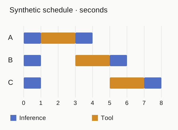
For three identical tasks, each with inference 1 s → tool 2 s → inference 1 s, a single admission slot yields 12 s. Admit all three while preserving one tool slot: first inference stages overlap during seconds 0–1, tools run during 1–3, 3–5 and 5–7, and final inference stages finish at 4, 6 and 8 s. Makespan becomes 8 s without accelerating any operation. Mean completion is 6 s, versus 8 s under serial admission. This is an original deterministic example with unconstrained inference parallelism, not a measured GPU result.
The resource bound is 6 s and the longest individual path is 4 s, so the generic bound is 6 s. The actual 8 s reflects the initial release delay and the last inference stage. That gap is why a utilization dashboard alone cannot certify an optimal schedule. A realistic server also has batching effects: increasing concurrency can lengthen individual calls while decreasing total batch duration.
A reference architecture with two independent gates
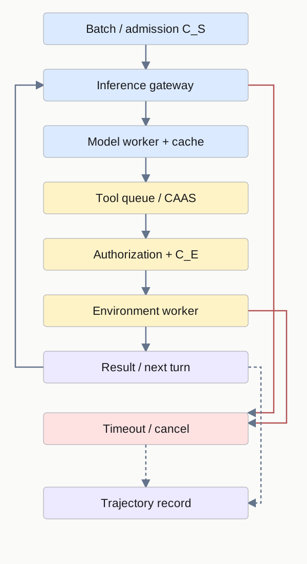
An admission controller owns
A trajectory label is an affinity hint, never an authorization credential. Before dispatch, validate tenant, tool capability, arguments, deadline and cancellation state. Returning a tool result releases only the next dependent turn; it does not create permission for a new action. Keep cache keys separated by authorized sharing scope and model/tokenizer configuration. Cross-tenant reuse requires a separate security decision; a matching label is insufficient.
Use a bounded pending queue and admission backpressure. On timeout, record an explicit uncertain or failed outcome. If a side effect might already have happened, inspect its operation ID or state before retrying; releasing a semaphore is not rollback. Cancellation must stop queued work and propagate to running calls where supported. Repeated retries need a separate budget and backoff. Store the checkpoint before making the next stage ready. These reliability rules are proposed engineering requirements, not claims tested by the paper.
Hybrid cache capacity: two pools can bottleneck one another
For an ordinary attention model, saved keys and values grow with cached token length. A hybrid model can additionally retain a recurrent summary for a trajectory. Reusing a prefix may require both kinds of state. A large empty KV pool is useless if the recurrent-state pool cannot retain the same trajectories. The paper therefore selects a workload-informed allocation at deployment; it does not resize these pools dynamically during the batch.
Let M be memory available after weights and runtime reservations,
An original example reserves 12 GiB for caches, with
Routing and scheduling preserve opportunities, not guarantees
Worker affinity avoids repeatedly rebuilding a growing prefix, but strict affinity can overload one replica while another is idle. The paper’s load-bounded consistent hashing starts from a trajectory’s home worker and permits spillover when the home worker exceeds a load threshold. It uses observed in-flight requests rather than predicting future token counts. A spill may intentionally sacrifice reuse to avoid a longer queue; cache-hit rate is therefore an intermediate metric, not the final objective.
Inside a worker, routing-prefix scheduling uses recent trajectory labels to narrow priority-related prefix lookups. A remembered label is not evidence that the underlying GPU state is still resident. Conversely, dropping a label does not delete the cache. This distinction matters operationally: telemetry must separately count routing affinity, actual prefix reuse, uncached prefill tokens, queue delay and terminal completion. Otherwise a high affinity percentage can conceal expensive recomputation.
For a pure attention deployment, recurrent-state partitioning is irrelevant, but the routing trade-off remains. For shared-cache systems, network transfer cost enters the choice; this paper’s worker-local reuse model does not establish an optimum for cross-worker cache migration. For heterogeneous workers, request count alone is a weak load estimate. Consider service demand and capacity before adopting a homogeneous-worker routing rule.
Advancing observed long chains without knowing the future
After capacity separation, tool ordering determines which trajectories reveal their next stages. CAAS groups job arrivals into bands of width B seconds. Within the oldest band it prefers greater completed inference depth, then a bucketed shorter observed mean inference duration, then FIFO sequence. The completed-turn count includes the turn that generated the pending tool job. Priorities are fixed on enqueue. The scheduler does not inspect future trace lengths. In the priority tuple,
Suppose B=30 s and the duration bucket is 1 s. Job A arrives at 61 s after 4 turns averaging 2.2 s: its key begins (2,−4,3). Job B arrives at 59 s after 1 turn averaging 1 s: (1,−1,1). B wins because its arrival band is older. Job C arrives at 62 s after 7 turns averaging 3.1 s: (2,−7,4), so C precedes A within band 2. Depth matters only after the arrival-band comparison.
Depth is a heuristic for possible long remaining work, not a critical-path oracle. A task that has already completed many turns may actually be almost done; another at turn one may have a huge future. Small B approaches arrival order; large B gives depth more influence. Earlier bands limit repeated overtaking, but this is not a guarantee of tenant fairness, deadlines or bounded waiting under stalled operations. Use separate quotas and aging/SLO rules when those are requirements.
What the published numbers do—and do not—show
The November 12 v1 technical report evaluates Ling-3.0-Flash and Ling-3.1-Flash using H20 deployments and multiple agent workloads. Its headline 10.4%–65.0% makespan reduction belongs to combined configurations, not to CAAS alone. In the live MCP-Atlas comparison, the authors average three runs of 500 tasks. The table below reproduces selected numerical facts with attribution; it is not a Token Lab benchmark.
For Ling-3.0, 466.1 → 168.2 min is a 63.9% reduction from inference optimizations plus separated admission. Switching only the environment policy in that optimized setup gives 168.2 → 163.0 min, a further 3.1%. Relative to the original baseline, the combined reduction is 65.0%. Adding 63.9% and 3.1% is wrong because the denominators differ. Live runs include retries and terminal failures. That does not establish behavior under an injected retry storm or adversarial multi-tenant load.
Replay holds stage sequences and environment durations fixed but performs actual inference. It measures execution efficiency, not whether generated actions remain semantically correct. Live experiments complement replay but include stochastic differences in trajectories. The reported final-5% interval can increase against the narrow-admission baseline even while makespan drops: different tasks remain in the tail. Compare absolute batch completion as well as cohort composition; do not optimize the tail interval in isolation.
| Model | Baseline | Opt-FCFS | Opt-CAAS |
|---|---|---|---|
| Ling-3.0 | 466.1 | 168.2 | 163.0 |
| Ling-3.1 | 333.5 | 140.5 | 128.5 |
arXiv:2611.16661v1 · Table 3https://arxiv.org/html/2611.16661v1#S5.T3
Where this belongs in a production system
First decide which service owns the objective. For a nightly evaluator, minimize time to a complete valid report at a fixed hardware and API budget. For RL, also account for policy-version freshness: a faster collection batch is not automatically a better learning update if trajectories are stale or selected unfairly. For user-facing agents, constrain p95 response latency and tenant service before optimizing batch throughput. Never drop failures from the denominator to make completion look better.
Separate CPU-limited shell execution, rate-limited external APIs and exclusive simulators into resource classes; one homogeneous
Open problems include online capacity adaptation, robust load estimation for heterogeneous workers, cache transfer economics, fairness across tenants and retry-amplification control. A useful deployment sequence is an instrumented baseline, a reversible configuration change, then a guarded rollout with the original scheduler available. Do not let a learned or heuristic scheduling score bypass permissions, deadlines or cancellation. The validation plan and executable teaching model follow only after these mechanisms and boundaries are clear.
Practice and validation
Run Python 3.11+ with no packages, API keys or network. The first case verifies the 12 s versus 8 s calculation. The seeded 50-trajectory case compares FCFS and the published CAAS priority rule on identical synthetic traces. The implementation has unlimited parallel inference with fixed delays, homogeneous non-preemptive tool slots and one outstanding tool stage per trajectory. It does not implement GPU batching, cache eviction, routing, real tools, failure recovery or the authors’ system.
agent-batch-scheduler.pypython3 agent-batch-scheduler.pyExpected output (seed 17): the simple case is 12.0/8.0 s under both policies; mixed FCFS is 427.0 s and CAAS is 411.0 s. Final-5% intervals are 28.0/2.0 s; mean completion is 221.30/220.58 s. These are synthetic simulator outputs, not predictions for your deployment. With only three tasks, the discrete 95% quantile is the final task, so its tail interval is zero and uninformative.
Python · agent-batch-scheduler.py
"""Token Lab synthetic scheduling lab. Python 3.11+, standard library only.
No model, API, tools, GPU or external environment is called.
Inference stages have fixed durations and unlimited parallel capacity.
This is an independently written teaching model, not the paper's evaluator.
"""
from dataclasses import dataclass
from heapq import heappush, heappop
from math import ceil, floor, isfinite

@dataclass(frozen=True)
class Trace:
    inference: tuple[float, ...]
    environment: tuple[float, ...]
    def __post_init__(self):
        assert len(self.inference) == len(self.environment) + 1
        assert all(isfinite(x) and x > 0 for x in self.inference + self.environment)


def run(traces, samples=4, environments=1, policy="fcfs", band=30.0, bucket=1.0):
    assert samples > 0 and environments > 0 and band > 0 and bucket > 0
    assert policy in {"fcfs", "caas"}
    events, pending, completed, spans = [], [], {}, []
    active = busy = next_task = serial = 0
    observed = [0.0] * len(traces)
    max_busy = 0
    def schedule(end, kind, task, turn):
        nonlocal serial
        serial += 1
        heappush(events, (end, serial, kind, task, turn))
    def admit(now):
        nonlocal active, next_task
        while active < samples and next_task < len(traces):
            task = next_task
            next_task += 1
            active += 1
            schedule(now + traces[task].inference[0], "inference", task, 0)
    admit(0.0)
    while events:
        now = events[0][0]
        # Process simultaneous completions before choosing the next environment job.
        while events and events[0][0] == now:
            _, _, kind, task, turn = heappop(events)
            trace = traces[task]
            if kind == "environment":
                busy -= 1
                schedule(now + trace.inference[turn + 1], "inference", task, turn + 1)
            else:
                observed[task] += trace.inference[turn]
                if turn == len(trace.environment):
                    completed[task] = now
                    active -= 1
                else:
                    serial += 1
                    key = (serial,) if policy == "fcfs" else (
                        floor(now / band), -(turn + 1),
                        ceil(observed[task] / (turn + 1) / bucket), serial)
                    heappush(pending, (key, task, turn, now))
        admit(now)
        while pending and busy < environments:
            _, task, turn, arrival = heappop(pending)
            end = now + traces[task].environment[turn]
            spans.append((task, turn, arrival, now, end))
            busy += 1
            max_busy = max(max_busy, busy)
            schedule(end, "environment", task, turn)
    assert len(completed) == len(traces) and not pending and busy == active == 0
    ordered = sorted(completed.values())
    t95 = ordered[ceil(.95 * len(ordered)) - 1] if ordered else 0
    end = ordered[-1] if ordered else 0
    return {"makespan": end, "tail5": end - t95,
            "mean_completion": sum(ordered) / len(ordered) if ordered else 0,
            "completed": completed, "spans": spans, "max_busy": max_busy}


def checks():
    short = Trace((1., 1.), (2.,))
    assert run([short], samples=1)["makespan"] == 4
    assert run([short] * 3, samples=1)["makespan"] == 12
    assert run([short] * 3, samples=3)["makespan"] == 8
    for policy in ["fcfs", "caas"]:
        r = run([short] * 3, samples=3, environments=2, policy=policy)
        assert r["max_busy"] <= 2 and r["makespan"] == 6
        assert sum(e-s for _, _, _, s, e in r["spans"]) == 6
    # Earlier arrival bands outrank later bands regardless of observed depth.
    assert (0, -1, 5, 1) < (1, -100, 1, 2)
    try:
        Trace((1.,), (2.,))
    except AssertionError:
        pass
    else:
        raise AssertionError("invalid dependency chain accepted")
    return short

if __name__ == "__main__":
    short = checks()
    print("checks=passed")
    for policy in ["fcfs", "caas"]:
        for capacity in [1, 3]:
            r = run([short] * 3, samples=capacity, policy=policy)
            print(f"{policy} C_S={capacity} C_E=1 makespan={r['makespan']:.1f}s")
    # A broader synthetic comparison, with identical traces for both policies.
    import random
    rng = random.Random(17)
    traces = []
    for _ in range(50):
        turns = rng.choice([1, 2, 8, 16])
        traces.append(Trace(tuple(float(rng.randint(1, 4)) for _ in range(turns+1)),
                            tuple(float(rng.randint(1, 6)) for _ in range(turns))))
    for policy in ["fcfs", "caas"]:
        r = run(traces, samples=20, environments=3, policy=policy)
        print(f"{policy} mixed makespan={r['makespan']:.1f}s tail5={r['tail5']:.1f}s "
              f"mean={r['mean_completion']:.2f}s")
For a fair comparison, keep the same traces, submission order,
Original interview exercises—not company interview questions
Why can TPOT become worse while the batch finishes sooner?
Hint
Distinguish per-call competition from overlap across tasks.
Answer and analysis
Higher admitted concurrency may slow each active decode while keeping more independent stages in flight. The appropriate objective is constrained makespan, with a separate latency SLO if needed. Report both rather than declaring either universally better.
Does the 65% headline measure CAAS alone?
Hint
Choose the baseline that differs in exactly one intervention.
Answer and analysis
No. For live Ling-3.0 MCP-Atlas, compare 168.2 with 163.0 min for the incremental policy effect: about 3.1%. Comparing 466.1 with 163.0 measures the combined configuration. These comparisons have different denominators.
What happens if all trajectory labels are retained but the cache is evicted?
Hint
A routing hint is not storage state.
Answer and analysis
Affinity still directs calls, but prefill recomputation rises. Measure actual cached tokens and uncached work. Recover by rebuilding authorized context; never assume a label makes stale or cross-tenant data valid.
A tool times out after submitting a payment. Should the scheduler immediately retry?
Hint
Separate resource accounting from external side effects.
Answer and analysis
No automatic blind retry. Record uncertainty, reconcile the operation ID with the payment system and apply an idempotency contract. Semaphore release does not undo the payment. A scheduling speedup cannot justify duplicate business actions.
Scoring: 1—names the metric; 2—distinguishes queues, admission and execution; 3—derives the numerical example and runs the code; 4—designs controlled comparisons and explains a regression; 5—adds failure semantics, tenant constraints and a justified production rollout. Mastery requires all five abilities, not reading time alone.
Predict, test and keep evidence
Before revealing an answer, predict one result. After the exercise, record the discrepancy and a transfer test. Saved locally across language editions.
Open notebook / export / clear →The mathematical review scope is recorded per lesson. It does not establish empirical paper reproduction; report suspected errors in your notes. Review scope
References and further learning
Primary paper by Wei Feng et al., Ling Team, Ant Group. Version v1 is CC BY 4.0; formulas, method descriptions and the selected data table are attributed adaptations. Diagrams, numerical examples and simulator are original Token Lab teaching material. No implementation repository for the paper was verified in this review; the local simulator must not be presented as the authors’ code.
- arXiv · abstract / v1https://arxiv.org/abs/2611.16661v1
- arXiv · PDF / v1https://arxiv.org/pdf/2611.16661v1
- arXiv · full HTML / v1https://arxiv.org/html/2611.16661v1
- CC BY 4.0https://creativecommons.org/licenses/by/4.0/
- SGLang · sourcehttps://github.com/sgl-project/sglang
- Stanford CS329Z · Engineering AI Agentshttps://cs329z.stanford.edu/