AI infrastructure in 2026: from fast chips to useful, reliable capacity
Follow a request through admission, prefill, KV memory, decoding, tools and recovery; connect capacity and cost to frontier hardware and market evidence.
出典とバージョン
Contents · lifecycle and reference chapters
この記事の目次
インフラ:要求の経路を追う
この独自事例では請求書アシスタントを追います。テナント内の資料を読み支払いを提案しますが、実行には別途正確な認可が必要です。場面と実験は合成教材であり、実際の導入事例ではありません。
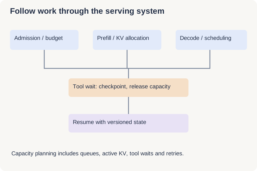
一つの要求から発票エージェント基盤を理解する
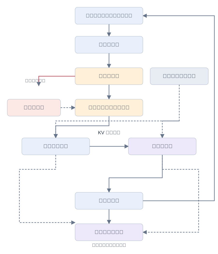
社員がINV-42の遅延理由と条件付き支払い準備を依頼します。助手はテナント資料と状態を照会し説明・提案しますが、実行には別の正確な承認が必要です。これは合成教材であり特定企業の実装ではありません。基盤は流暢な文ではなく永続的な業務を支えます。
要求は認証ゲート、ワークフロー、検索保存、推論、ツールゲート、業務系を横断します。読み取りは通常再試行できますが、支払い送信のタイムアウトは結果照合が必要です。モデルプロセスを取引の正本にせず、永続状態に未完了段階、使用根拠、確定状態を残します。
ハードウェア選定前に到着率、突発、入出力token分布、タスク当たり呼び出し、検索分岐、ツール遅延、締切を定義します。対話と背景照合は別です。毎秒10要求でも200tokenの回答と8回の長文呼び出しは違います。非決定的推論を繰り返さず回復できる状態を定義し、会話記録をそのままチェックポイントとみなさないでください。
段階1:受け入れ、文脈構成、資源予算
ゲートは入列前に認証とテナント解決を行います。レート制限は共有サービスを保護し、受け入れ判定は締切を満たせるか判断します。無限キューへ入れ遅すぎる回答を返すより早い拒否・延期が適切な場合があります。
指令、ツールschema、根拠、履歴、最大出力の予算を確保します。文脈上限は埋める目標ではありません。関連し許可された資料を選び、切り詰めでも必要方針と出典を保持します。資料のため承認条件を削除してはいけません。
受け入れは推定token、後の精算は実使用量で行います。要求数以外にテナント並行数と占有量を制限します。少数の巨大入力もメモリを独占します。取消を検索と推論へ伝播します。合成例の稼働24、待ち48、待機期限2秒は推奨値ではなく明示的境界です。平均遅延だけでなく第二テナントの進行も守ります。
段階2:Prefill、decode、KVメモリとスケジューリング
検索後は入力処理をしてからtokenを生成します。長い入力は最初のtokenを遅らせ、長い出力はその後もdecode容量を占有します。最初のtoken、token間、最後のtoken、業務全体完了の遅延を区別します。
通常のKVメモリ概算は2×層数×KVヘッド数×ヘッド次元×token数×要素バイト数を常駐系列について合計します。32層、KVヘッド8、次元128、8192token、2バイトなら一系列1 GiB、16系列16 GiBです。重み、活性、断片化、その他状態は別です。GQAで問い合わせヘッド数を代入してはいけません。
バッチは実行を共有しますが、形成待ちが遅延を増やします。終了時刻が異なるため、稼働系列とメモリは動的です。長いprefillの分割はdecode応答を守る可能性がありますが、カーネル、ハードウェア、負荷に依存します。均一バッチから実負荷を推測しないでください。
vLLMのprefix cachinghttps://docs.vllm.ai/en/stable/features/automatic_prefix_caching/は共通接頭辞の計算を再利用します。繰り返しprefillを減らしても新しい出力生成は必要です。コールドとウォームの負荷及び分離条件を区別します。
容量購入前にボトルネックを区別します。Prefillは入力全体の注意力と前向き計算を行い、decodeは重みとキャッシュを繰り返し読み、各系列から少数の新しいトークンを作ります。制約はバッチ、文脈、カーネル、ハードウェア次第です。テンソル並列は通信を、パイプライン並列は段間の空き時間を生みます。複製による容量増加にはモデルが収まり負荷を分配できる条件が必要です。
Prefillとdecodeの分離はKV転送を必要とします。1 GiBのキャッシュを理想的な25 GiB/sで転送しても、バイトだけで最低40 msかかり、プロトコル、競合、引き継ぎが上乗せされます。実測ではなく算術下限です。転送と遊休容量の費用が削減できる干渉を上回れば分離は不利です。量子化も対応カーネルが必要で、低ビット化だけで高速化や品質維持を証明できません。
段階3:ルーティングと代替は挙動を変える
単純照会を安いモデル、紛争を高能力モデルへ送れても、振り分け自体が誤ります。難題を単純と判定したり全件を高価な経路へ送ったりします。判断、モデル・指令版、予算を残して回帰を帰属できるようにします。
障害時の代替モデルはツール構文、文脈、指令順守、拒否が異なります。アダプターは構文を揃えても業務同等性を保証しません。有効化前に挙動の根拠を持ち、同じ認可・承認境界を守ります。
サーキットブレーカーは失敗依存先への反復を、バックオフと予算は負荷増幅を抑えますが、副作用の有無は示しません。推論と業務の再試行を分離します。新提案は再支払いの許可ではありません。チェックポイントは論理操作と状態を保持します。主経路、代替、安全な棄権の意味・費用・失敗条件を比較し、稼働率だけで選びません。
段階4:キュー、費用、有効な仕事をつなぐ容量計画
容量計画は負荷増加に伴う合格スループットと遅延のサービス曲線から始めます。飽和付近では平均GPU利用率が正常に見えても待ち時間が急増します。token生成数が増えて締切内完了が減る場合もあるため、品質と遅延条件を定めます。
安定系のLittleの法則は平均在途数を到着率と平均滞在時間に結びます。毎秒8件、平均3秒なら24件です。安定条件下の会計関係であって、24枠でp99を満たす保証ではありません。突発、処理時間の分散、相関障害も重要です。
合成例で1000要求に20ドル、800件が合格なら一要求0.02ドル、合格一件0.025ドルです。安い経路で16ドルでも合格500件なら0.032ドルに悪化します。予約容量、遊休、保存、ネットワーク、人の確認費用も総費用へ分けて計上します。
一つのタスクは一回の呼び出しではありません。毎秒10タスク、平均3回のモデル呼び出しなら再試行前に30回/秒です。各呼び出しの10%が独立に追加一回を必要とするなら33回/秒になります。合成の一回再試行モデルであり、相関障害や再帰ループには当てはまりません。タスク単位と全体の再試行予算を制限します。
拡張には起動時間と状態が関係します。重み読み込みに数分かかるなら数秒の突発には既存余力、キュー、拒否で対応します。後から準備できる複製は間に合いません。GPU利用率だけでなくキュー滞留時間、稼働トークン、測定済み容量を用います。品質と公平性を保ち締切内完了を増やして初めて容量増加が有効です。
段階5:リリース、回復、説明可能な運用
リリースは重みだけでなくtokenizer、指令、schema、索引、量子化、推論エンジン、振り分けを含みます。版と互換性を管理します。事故再現にはモデル名に加えて歴史的文書やツール応答が必要な場合があります。
オフライン確認、操作不能なshadow、限定canaryの順に進めます。負荷は変化するため同期の基準と比較します。ロールバックはワークフローとschemaの互換性を戻しても確定支払いを取り消しません。不可逆操作を実験するには明示の承認と補償方針が必要です。
ワークフロー記録とキャッシュの回復時間・許容喪失を分けます。KV再計算と承認証拠・確定状態の喪失は違います。回復時も取消、権限撤回、冪等性を維持します。負荷モデル、実測容量、依存回復計画、タスク成果につながるリリース報告を残します。ハードウェアや企業選定は実測ボトルネックと総リスク・費用から判断します。
How the four disciplines fit together
Security determines which actions are permitted. Infrastructure executes work within capacity and failure constraints. Observability preserves evidence of what happened. Evaluation tests whether a change improves the outcome under a declared contract. None substitutes for the others.
仕組み・研究・市場背景 — 以下の参考資料は英語です
The following chapters provide the mathematical examples, experiments, research papers and dated company evidence behind the operational story. Return to the lifecycle when deciding where each mechanism belongs.
1. The unit of progress is a completed workload
An AI infrastructure stack turns electricity, silicon, software and operational labor into training runs or useful responses. A faster accelerator is only one input. A customer experiences the time to a correct answer; an operator pays for reserved capacity, idle time, retries and failures as well as successful computation. The important question is therefore not “which chip has the largest number?” but “what bottleneck prevents this workload from meeting its service objective?”
Definitions. An accelerator is a processor optimized for selected computations. HBM is high-bandwidth memory close to the accelerator; it is not interchangeable with host RAM or remote storage. Scale-up interconnects connect processors within a tightly coupled system; scale-out networking joins systems. A service-level objective (SLO) specifies a measurable target such as a latency percentile. Goodput is the rate of useful completions satisfying specified constraints, rather than every generated token or attempted request.
Before this lesson: understand that matrix multiplication creates reusable parallel work, while autoregressive generation has a dependency between output steps. Understand a byte, a second and a watt: power measures a rate of energy use, and capacity in GiB says nothing by itself about transfer rate. Finally, distinguish average latency from a tail percentile. An average can improve while the slowest users experience worse service. Review attention and KV-cache correctness if those distinctions are unfamiliar.
Learning goals: draw the system boundary; calculate a cache budget with units; identify a misleading benchmark comparison; explain why an acquisition adds an engineering capability; and design a repeatable serving experiment. The company map below is selective, not a complete procurement recommendation or a claim that every listed product is available in every region.
2. Read the stack from the workload down
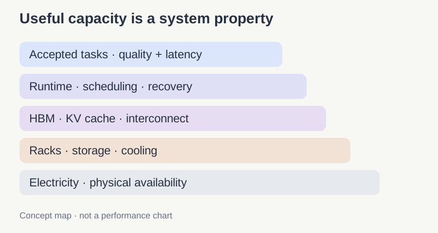
Start at the application. A short autocomplete request, a long-document question and an agent executing twenty tool steps have different prompt lengths, output lengths and interruption patterns. A speech assistant needs predictable delay; an overnight research job may accept queuing. One aggregate “tokens per second” metric conceals these differences. Record the request distribution before choosing a runtime or hardware platform.
The serving runtime schedules requests and manages state. Continuous batching can admit new work as other requests finish, but mixing a large prompt with latency-sensitive decoding can create interference. Cache allocation determines how many active sequences fit. Parallelism then distributes weights and work across processors. If a model requires frequent collectives or expert routing, communication may erase the benefit of additional compute.
The rack supplies the physical constraints: memory channels, interconnect topology, cooling and electrical delivery. A training job also needs dataset throughput and durable checkpoints. A data pipeline can starve expensive processors; a recovery procedure can waste a large fraction of a run even when individual kernels are fast. Capacity planning must include failed jobs and reloading weights, not just the steady state.
Our engineering interpretation is that differentiation increasingly comes from coordinating these layers. An efficient kernel does not repair a slow scheduler; a faster network does not fix an inaccurate low-precision model; an available GPU does not imply an energized rack. This is why infrastructure is both a distributed-systems problem and an industrial deployment problem.
業界構造:制御点・購買者・競争
業界資料の確認日:2026年11月8日。製品文書は機能の提供を示すもので、独立した効果測定ではありません。競争上の見解と未解決機会は Token Lab の分析です。合成例は企業の実測値ではありません。
AI基盤:容量・ワークフロー・責任を誰が持つのか
2026年11月8日に確認した業界分析です。公式資料で製品範囲と取引の節目を確認し、競争上の結論は独自の解釈として示します。市場シェア順位や独立性能試験ではありません。日付のない製品ページは確認日、日付付き資料は公開・更新日を示します。
市場を責任の連鎖として読む
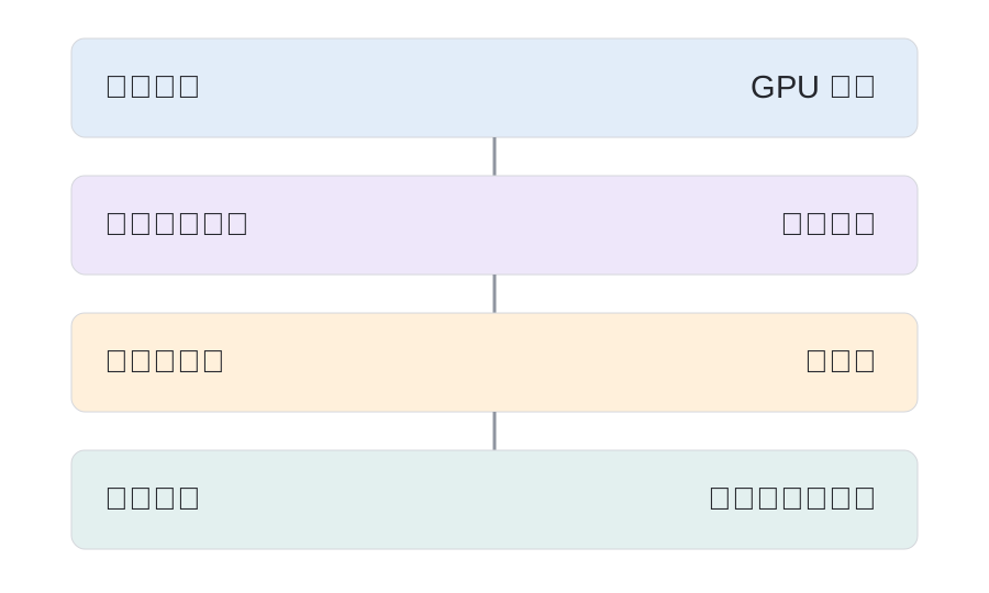
企業アシスタントを保存文書からタスク完了まで追います。データ基盤は許可された証拠を、GPUクラウドは容量を供給し、推論運用者が応答を生成し、アプリが許される操作を決めます。各層は別のボトルネックを解消します。すべてを交換可能なAIクラウドと見ると、購入者、利益構造、安全責任が見えません。以下は市場占有率の実測や投資助言ではなく分析です。私設エンドポイントが通信を守っても、過剰権限のアプリは他テナントの記録を漏らせます。
参照構成:遅延とメモリ制約下の推論
分離型プリフィル/デコードを選び費用を可視化していますが、全配置への要件ではありません。受付時にトークンと同時実行予算を予約します。入力処理後、KV 状態を互換デコード実行器へ転送します。登録庫は固定版のモデル制品を供給します。両群は指標を出し、取消と期限は予約解放のため実行器まで伝達します。
特化の利点が直列化、通信、調整費を上回る必要があります。同居型は転送不要で小規模負荷に適する場合があります。プレフィックス共有ではモデル、形式、隔離境界を合わせます。キュー長と待機時間を制限し、増設で飽和が即解消するとは考えません。待機、初回トークン、生成間隔、KV ピークを分けて観測します。
企業と製品の位置付け
選択的な業界地図であり、市場シェア順位や認証ではありません。対象範囲は版、統合、配置、強制モードによって異なります。
NVIDIA
- 所有者・組織
- NVIDIA
- 制御点
- アクセラレータ・接続・オーケストレーション
NVIDIAは、GPUを有用なサービスへ変えるための補完的なハードウェアとソフトウェアを提供します。Dynamoは分散推論、Run:aiはワークロード配分を扱います。2026年10月13日、4つのモジュールを含むRun:ai全体がオープンソース化されました。分析上、汎用スケジューリング機能には価格圧力が生じ、統合と運用支援には価値が残ります。資源割当やGPU共有はアプリの認可を成立させず、強いテナント分離の証明にもなりません。
NVIDIA: full Run:ai platform open-source release ↗https://developer.nvidia.com/blog/nvidia-runai-is-now-open-source-as-part-of-nvidia-dsx-ai-factory-platform · NVIDIA Dynamo ↗https://www.nvidia.com/en-us/ai/dynamo/
AWS
- 所有者・組織
- Amazon
- 制御点
- クラウド・マネージドモデルAPI
AWSは既存のID、課金、運用システムを利用する企業に強みがあります。BedrockはモデルへのマネージドアクセスとIAMを組み合わせ、速度だけでなく調達や統合にも利点があります。安全性は責任共有モデルに従い、顧客は資格情報、データ、下流ツールの権限を限定する必要があります。モデルを呼び出せるIDが、提案された全操作を実行できるわけではありません。クラウドブランドではなく、具体的な構成の制御を評価します。
Amazon Bedrock: data protection and shared responsibility ↗https://docs.aws.amazon.com/bedrock/latest/userguide/data-protection.html · Amazon Bedrock: invocation permissions ↗https://docs.aws.amazon.com/bedrock/latest/userguide/inference.html
Microsoft Foundry
- 所有者・組織
- Microsoft
- 制御点
- 企業AIコントロールプレーン
Microsoftはモデル、エージェント開発、接続先Azure資源を企業管理構造にまとめます。購入側は既にEntraやAzure利用契約を持つ場合が多く、調達とガバナンス統合が重要です。Foundryには資源・プロジェクトのロール、マネージドID、プライベートネットワークがあります。ただし全依存先が自動的に隔離されるわけではなく、AIゲートウェイやデータサービスも個別設定が必要です。機微な操作の認可と実際の結果の照合はアプリ側に残ります。
Microsoft Foundry architecture ↗https://learn.microsoft.com/en-us/azure/foundry/concepts/architecture · Microsoft Foundry network isolation ↗https://learn.microsoft.com/en-us/azure/foundry/how-to/configure-private-link
Google Cloud
- 所有者・組織
- Alphabet
- 制御点
- AI・データ・クラウド統制
Google Cloudは企業データとマネージドAIの接点で競争します。ID、サービス境界、暗号化・鍵制御を組み合わせますが、対応範囲はサービスごとに違います。データ所在地の条件は一部のグラウンディングやRAG機能を区別します。分析上、既存データとの統合はモデル一覧より強い競争基盤になり得ます。一つのAIサービスの承認を全接続機能の適合性へ広げず、処理経路と機能ごとに確認する必要があります。
Google Cloud service-specific data residency ↗https://cloud.google.com/terms/data-residency · Google Cloud: securely deploying AI ↗https://cloud.google.com/blog/products/identity-security/mastering-secure-ai-on-google-cloud-a-practical-guide-for-enterprises/
CoreWeave
- 所有者・組織
- CoreWeave
- 制御点
- GPUクラウド・開発ワークフロー
CoreWeaveは専門的なGPU容量を供給し、Weights & BiasesとOpenPipeを通じてソフトウェアへ拡張しています。顧客は確実な容量提供と、開発から学習・配信までの短い経路を買います。実験や事後学習のワークフローを持つことは継続利用と計算需要を高め得ますが、資本集約性や集中リスクは消えません。基盤の保護とアプリの権限は別です。買収完了は所有権の証拠であり、統合成功やモデル品質、安全性の証明ではありません。
CoreWeave completes Weights & Biases acquisition ↗https://www.coreweave.com/blog/coreweave-completes-acquisition-of-weights-biases · CoreWeave 2025 Form 10-K ↗https://www.sec.gov/Archives/edgar/data/1769628/000176962826000104/crwv-20251231.htm
Nebius
- 所有者・組織
- Nebius Group
- 制御点
- GPU容量・本番クラウド
Nebiusは大規模専用容量、マネージドクラウド、本番ガバナンスを組み合わせます。Microsoftとの契約は、巨大クラウドが競争相手でも顧客でもあり得る構造を示します。2025年の発表は、展開と可用性を条件に2031年まで約174億ドル、追加拡張の可能性を示しました。年次売上や受領済み現金ではありません。IAMと基盤統制は企業導入を助けますが、顧客データ方針やエージェントの操作権限は容量契約では解決しません。
Nebius Cloud 3.6 governance release ↗https://nebius.com/newsroom/nebius-ai-cloud-3-6-strengthens-developer-experience-and-governance-for-production-operations · Nebius–Microsoft agreement ↗https://www.sec.gov/Archives/edgar/data/1513845/000110465925088312/tm2525580d1_6k.htm
Together AI
- 所有者・組織
- Together AI
- 制御点
- オープンモデル推論・展開
Togetherはオープンモデルを使いながら配信運用をすべて自作したくないチーム向けです。専用エンドポイントは隔離GPUを予約し、展開や性能管理を提供します。経済性の分岐は利用率です。安定需要にはGPU時間予約、不規則需要にはトークン課金が適する場合があります。地域選択はプランと設定に依存します。隔離は提供者のアクセス問題を消さず、API互換性も運用上の移植性を保証しません。実モデルと要求分布で検証します。
Together dedicated model inference ↗https://www.together.ai/dedicated-model-inference · Together EU deployment requirements ↗https://support.together.ai/articles/8079447813-eu-data-centers-and-dedicated-model-deployment
Fireworks AI
- 所有者・組織
- Fireworks AI
- 制御点
- 推論エンジン・フリート運用
FireworksのSovereignは顧客所有GPU上で配信スタックを運用し、基盤所有と推論ソフトウェア・運用を分離します。顧客がネットワーク境界を管理し、Fireworksは監査可能な初期設定用資格情報と限定的なコンポーネントIDを説明しています。BYOCは提供者アクセスがゼロという意味ではありません。任意のクラウドへの負荷移送はデータ境界を変えます。性能改善の宣伝値は独立比較ではなく、競争力は再現可能な効率と運用実績で判断します。
Fireworks Sovereign shared responsibility ↗https://fireworks.ai/product/sovereign · Fireworks enterprise controls and retention exceptions ↗https://fireworks.ai/solutions/for-enterprise
Baseten
- 所有者・組織
- Baseten
- 制御点
- カスタムモデル配信・展開
Basetenは複数のクラウド容量を使ってモデルを管理展開したいAI製品チーム向けです。2026年11月5日の安全実務文書は、論理分離した共有基盤、専用クラスタ、自社環境展開、ハイブリッド運用を区別します。これらは異なる信頼境界です。分析上、個別統合と確実な運用がモデル一覧以上の差別化になります。購入者は配置先、提供者アクセス、製品別の認証範囲を確認し、ある製品の認証を別製品へ自動適用してはいけません。
Baseten security practices ↗https://www.baseten.co/security-practices
Databricks
- 所有者・組織
- Databricks
- 制御点
- データ・モデル・業務アプリ基盤
Databricksは企業データをモデルやアプリへ変えるワークフローで競争します。MosaicMLは学習、Tabularはテーブル形式の相互運用性を加え、Neon技術は業務用PostgresのLakebaseを支えます。分析上、データ統合と蓄積された状態は重み以外の移行コストを生みます。統制は断片化を減らしても実行時認可の代わりにはなりません。カタログ権限は特定の外部決済を許可せず、トレース保存も決済完了を証明しません。
Databricks–MosaicML acquisition agreement ↗https://www.databricks.com/company/newsroom/press-releases/databricks-signs-definitive-agreement-acquire-mosaicml-leading-generative-ai-platform · Databricks–Tabular completed acquisition update ↗https://www.databricks.com/blog/databricks-tabular · Databricks Lakebase launch powered by Neon ↗https://www.databricks.com/company/newsroom/press-releases/databricks-launches-lakebase-new-class-operational-database-ai-apps
一つの構成に競争相手が共存する
各層は代替関係より補完関係になることがあります。企業は専門クラウドからGPUを借り、別提供者の推論スタックを載せ、データ統制は企業基盤に残せます。請求先は複数でも利用者には一つのサービスです。容量不足、展開停止、証拠へのアクセス不能、生成遅延、不正操作を別の事故として責任者へ対応付けます。統合は調整費用を下げても、単一契約が全構成要素の信頼性を均一にするわけではありません。新興企業の有望な入口は、供給者間で繰り返し壊れ、顧客の内製運用費が高い境界であり、GPU利用率の表示画面を増やすことではありません。
技術の要点:プリフィル・デコード・KV 予算
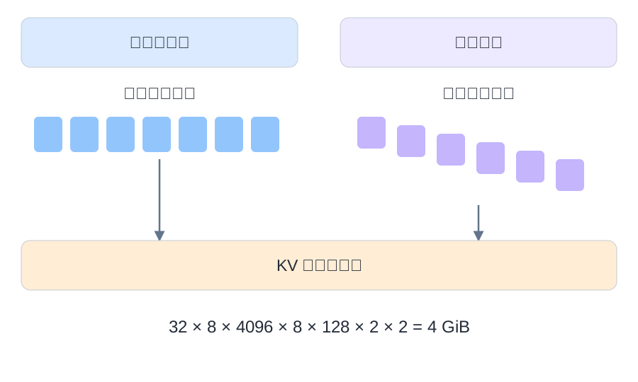
プリフィルは入力を処理して key/value 状態を構築し、デコードは新しいトークンの生成時に既存状態を繰り返し読みます。ボトルネックは負荷とハードウェア次第です。連続バッチ処理は利用率を改善しますが、過剰な並行処理は待ち時間とメモリ圧迫を増やします。両段階の分離は個別のスケジューリングを可能にする一方、KV 転送とネットワークの費用を伴います。必要な同時実行数で最初と後続トークンの遅延を満たす必要があります。
通常のキャッシュ容量は概ね 2 × 層数 × 有効系列数 × 系列ごとの保存トークン数 × KV ヘッド数 × ヘッド次元 × 要素バイト数です。順に32、8、4096、8、128、2なら4 GiBです。この合成例は重み、活性値、断片化、メタデータを除きます。グループ化クエリ注意は KV ヘッドを減らします。プレフィックス共有には再利用可能性と隔離条件が必要です。平均要求だけでなくピーク占有量を計画します。
容量・トークン・合格タスクの経済性
容量事業には機器、電力、納期、利用率のリスクがあります。推論ソフトは遅延と品質制約下の有効処理量、データ基盤は統合と継続利用で競争します。合成例では、Aは1,000要求に20ドル、合格800件で1件0.025ドルです。Bは16ドルでも合格500件なら0.032ドルです。Bは要求単価が安くても合格タスク単価は高くなります。節約を論じる前に遊休予約、再試行、データ移動、人手レビューを含め、タスク構成、品質基準、期限を揃えます。
別の合成例で容量リスクとソフトウェア利益を分けます。予約ワーカーが24時間当たり240ドルなら、有効稼働率80%では19.2時間が使え、実効単価は12.50ドルです。25%なら6時間しか使えず40ドルになります。予約価格は同じです。GPUの実際の見積もりではなく、稼働時間も有用な成果を保証しません。設備を所有する企業と顧客GPU上で運用するソフトウェア企業を比較する際、稼働率の約束、負荷の多様性、遊休費用の負担者が重要な理由です。この例から非公開企業の粗利益率は推定しません。
競争力と未解決課題が残る場所
オープンソースは利益を消すのでなく、その配分を変えます。Run:aiの4モジュールは調度機能の一部を標準化しますが、コミュニティ版に企業支援は含まれません。異種フリート復旧、方針準拠の複数提供者ルーティング、費用帰属、移行可能な証拠には機会が残り得ます。ルータは価格だけでなく地域、保持、品質、切替権限を守る必要があります。公開重みはIAM、評価履歴、展開状態の移植性を保証しません。責任境界とエクスポート経路を求め、予算責任者のいる反復障害か、基盤側が同梱できる修正かを検討します。
4. Electricity data: scale and uncertainty
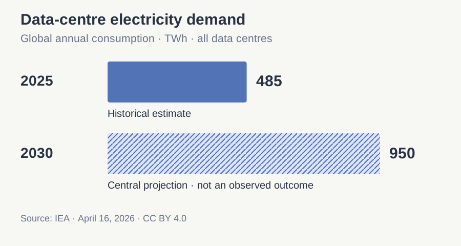
The IEA's 2026 update puts global data-centre electricity consumption at 485 TWh in 2025 and projects approximately 950 TWh in 2030 in its central outlook. These are not AI-only figures. The projected increase is roughly 1.96×, not an observation that consumption has already doubled. The report also identifies physical supply constraints, including HBM and power-system bottlenecks. IEA source, scope and assumptionshttps://www.iea.org/reports/key-questions-on-energy-and-ai/executive-summary.
Electricity demand is a useful scale indicator, not an AI capability metric. Lower energy per task can coexist with higher total consumption if adoption grows or tasks become more computationally intensive. A query that initiates repeated planning, retrieval and verification cannot be compared with a single short completion simply by counting user messages.
For a facility, distinguish IT load from total facility load. Power usage effectiveness is total facility energy divided by IT energy over the same measurement interval; it does not describe model quality. A lower value cannot compensate for wasted computation. For deployment decisions, measure energy per accepted task, peak power, cooling constraints and grid availability separately. A global TWh forecast cannot tell you whether a particular site can connect next quarter.
5. The technical frontier: what to optimize, and what can fail
Prefill and decode disaggregation
Prefill processes the input sequence and initializes the cache; decode repeatedly produces another token. Their operating points differ. DistServe studies separating the phases and selecting resource allocations around time-to-first-token and time-per-output-token constraints. Its original preprint appeared January 18, 2024; this reading pins arXiv v3, June 6, 2024. Abstracthttps://arxiv.org/abs/2401.09670v3 · PDFhttps://arxiv.org/pdf/2401.09670v3.
The useful inference is not “separation is always faster.” Moving cache state costs bandwidth and coordination. With short prompts or a constrained network, colocated execution can be simpler and competitive. Measure cache-transfer time, queue delay and both latency objectives. Hold offered load constant; a configuration that rejects difficult requests must not appear faster merely because it serves an easier subset.
KV cache as a first-class resource
Cache memory grows with active sequence tokens. Grouped-query attention reduces the number of key/value heads relative to query heads, changing memory requirements. Prefix caching can reuse shared prompt state, but tenant boundaries and cache keys must prevent unauthorized reuse. Offloading may increase capacity while adding transfer latency. These are separate interventions: benchmark each rather than calling all of them “cache optimization.”
Mixture of experts and interconnects
An MoE layer routes tokens to selected expert networks. Sparse activation reduces the arithmetic used per token relative to activating every expert, but weights still need storage and routing creates communication. Skewed expert demand can create hot spots. Compare expert placement, token imbalance, communication overlap and tail latency. Counting active parameters alone does not determine serving cost.
Quantization and speculative decoding
Lower precision can reduce memory traffic, but scales, outliers and unsupported kernels complicate the result. Verify downstream task quality and numerical behavior, not only model loading. Speculative decoding proposes multiple tokens and verifies them with a target model; useful acceleration depends on acceptance, proposal cost and verification efficiency. Keep the target distribution and implementation assumptions explicit. A fast draft with low acceptance can slow the full system.
Training reliability and elastic scheduling
Large training jobs coordinate many devices. More devices create more opportunities for hardware or software interruption. Checkpoint frequency trades useful computation against recovery exposure; storage contention can make frequent checkpoints expensive. For a shared cluster, optimize fairness and queue wait as well as accelerator occupancy. High utilization from low-priority work is not success if urgent jobs repeatedly miss deadlines.
買収・資本・戦略的影響
買収で変わる支配点
CoreWeaveはW&B契約を2025年3月4日に発表し、5月5日に完了しました。OpenPipeは9月3日発表、申告書は9月5日を交割に関連付けています。容量と開発・事後学習を接続する動きです。DatabricksのMosaicMLは2023年6月26日発表、7月19日完了で、約13億ドルには人材維持策を含みます。Tabularは2024年6月7日完了と公式ブログが確認しています。Neon技術のLakebaseは2025年6月11日公開ですが、Neonの厳密な法的交割日は本調査では確定していません。継続的ワークフローへの統合を示す一方、相互販売の成功は証明しません。発表、交割、製品統合は別の節目です。
製品・取引の一次資料
- NVIDIA: full Run:ai platform open-source release ↗https://developer.nvidia.com/blog/nvidia-runai-is-now-open-source-as-part-of-nvidia-dsx-ai-factory-platform ·
- NVIDIA Dynamo ↗https://www.nvidia.com/en-us/ai/dynamo/ ·
- Amazon Bedrock: data protection and shared responsibility ↗https://docs.aws.amazon.com/bedrock/latest/userguide/data-protection.html ·
- Amazon Bedrock: invocation permissions ↗https://docs.aws.amazon.com/bedrock/latest/userguide/inference.html ·
- Microsoft Foundry architecture ↗https://learn.microsoft.com/en-us/azure/foundry/concepts/architecture ·
- Microsoft Foundry network isolation ↗https://learn.microsoft.com/en-us/azure/foundry/how-to/configure-private-link ·
- Google Cloud service-specific data residency ↗https://cloud.google.com/terms/data-residency ·
- Google Cloud: securely deploying AI ↗https://cloud.google.com/blog/products/identity-security/mastering-secure-ai-on-google-cloud-a-practical-guide-for-enterprises/ ·
- CoreWeave completes Weights & Biases acquisition ↗https://www.coreweave.com/blog/coreweave-completes-acquisition-of-weights-biases ·
- CoreWeave 2025 Form 10-K ↗https://www.sec.gov/Archives/edgar/data/1769628/000176962826000104/crwv-20251231.htm ·
- Nebius Cloud 3.6 governance release ↗https://nebius.com/newsroom/nebius-ai-cloud-3-6-strengthens-developer-experience-and-governance-for-production-operations ·
- Nebius–Microsoft agreement ↗https://www.sec.gov/Archives/edgar/data/1513845/000110465925088312/tm2525580d1_6k.htm ·
- Together dedicated model inference ↗https://www.together.ai/dedicated-model-inference ·
- Together EU deployment requirements ↗https://support.together.ai/articles/8079447813-eu-data-centers-and-dedicated-model-deployment ·
- Fireworks Sovereign shared responsibility ↗https://fireworks.ai/product/sovereign ·
- Fireworks enterprise controls and retention exceptions ↗https://fireworks.ai/solutions/for-enterprise ·
- Baseten security practices ↗https://www.baseten.co/security-practices ·
- Databricks–MosaicML acquisition agreement ↗https://www.databricks.com/company/newsroom/press-releases/databricks-signs-definitive-agreement-acquire-mosaicml-leading-generative-ai-platform ·
- Databricks issuer release: MosaicML acquisition completed ↗https://www.prnewswire.com/news-releases/databricks-completes-acquisition-of-mosaicml-301881059.html ·
- Databricks–Tabular completed acquisition update ↗https://www.databricks.com/blog/databricks-tabular ·
- Databricks Lakebase launch powered by Neon ↗https://www.databricks.com/company/newsroom/press-releases/databricks-launches-lakebase-new-class-operational-database-ai-apps ·
- CoreWeave announces OpenPipe agreement ↗https://www.coreweave.com/news/coreweave-to-acquire-openpipe-leader-in-reinforcement-learning ·
- CoreWeave 2025 Q3 filing: OpenPipe closing ↗https://www.sec.gov/Archives/edgar/data/1769628/000176962825000062/crwv-20250930.htm ·
Source and maintenance notes
Primary links are placed beside the claims they support. Acquisition amounts retain their original basis; undisclosed values remain undisclosed. Product specifications and release statements are vendor disclosures, not comparative evidence from Token Lab. The diagrams and reference calculations are original educational material. Corrections should identify the section, source and proposed replacement; a source-access date is not a paper publication date.
All frontier research · Top Company Frontier · Editorial standards
実践と検証
実践:障害と負荷に対する基盤
提案後にモデルを止め、再起動後も承認待ちであることを確認します。ツール確認後にworkflowを止め、再試行前に照合します。会話は耐久チェックポイントではありません。
timeout、不正引数、モデル版不一致を注入し、有限試行、明示状態、主副同じ認可を要求します。同予算で安全な棄権と比較します。
長文、遅いツール、取消、突発、冷cache、障害を再生し、漏洩やキュー成長を観測できる時間実行します。ハード、精度、モデル、scheduler、softwareを記録し、同p95・合格率でthroughputを比べ、事前に戻す閾値を決めます。
稼働・待機上限を超え、明示過負荷、有限メモリ、別テナント進行を確認します。入力、出力、prefixを独立変更し冷热と隔離を区別、throughput、尾部遅延、最大メモリ、合格率を報告します。
地域障害、quota枯渇、遅い検索、承認待ち再起動から回復し取消、撤回、冪等性を確認します。ローカル実測と未証明の分散保証を区別します。
7. Reproduce a memory and cost budget
This is an original teaching calculation, not a vendor benchmark. Assume B active sequences, T cached tokens per sequence, L transformer layers, Hkv key/value heads, head dimension d and b bytes per stored value. K and V each have shape [B, Hkv, T, d] per layer. Ignoring allocation overhead and sharding:
For B=8, T=8192, L=32, Hkv=8, d=128 and b=2, the cache occupies 8 GiB. At 32768 tokens it occupies 32 GiB. Changing Hkv from 8 to 32 also gives 32 GiB at the shorter length. GiB means 2³⁰ bytes; device specifications expressed in GB need conversion before subtraction.
This is logical total cache size, not a claim about per-device allocation. Add weights, temporary activations, runtime reservations, fragmentation and any duplicated/sharded state. Weight quantization does not automatically quantize the cache. In a mixed-length batch, replace B×T with the sum of each active sequence's cached length.
At an illustrative $8 per hour and two accepted requests per second, the capacity cost is $0.001111 per accepted request. One accepted request per second doubles it. These hypothetical prices exclude network, storage, labor and idle reservations. “Accepted” should include a task-quality check and the agreed latency constraint; otherwise a faster but less useful system gets an unfair advantage.
Local capacity experiment
KV cache: 8.000 GiB for the stated eight-sequence configuration.
Predict the result before doubling the context length. No inputs leave your browser.
Download infra-capacity.py. Python 3.10+, standard library only; deterministic arithmetic, no random seed, network requests or model API. Run python3 infra-capacity.py.
"""Teaching arithmetic, not a GPU benchmark. Python 3.10+, standard library."""
from math import isclose


def kv_gib(batch, tokens, layers, kv_heads, head_dim, bytes_per_value):
    values = (batch, tokens, layers, kv_heads, head_dim, bytes_per_value)
    if any(not isinstance(x, int) or isinstance(x, bool) or x <= 0 for x in values):
        raise ValueError("All dimensions and bytes per value must be positive integers")
    return 2 * batch * tokens * layers * kv_heads * head_dim * bytes_per_value / 2**30


def cost_per_success(hourly_cost, accepted_per_second):
    if hourly_cost < 0 or accepted_per_second <= 0:
        raise ValueError("Nonnegative cost and positive accepted throughput required")
    return hourly_cost / (3600 * accepted_per_second)


if __name__ == '__main__':
    small = kv_gib(8, 8192, 32, 8, 128, 2)
    long = kv_gib(8, 32768, 32, 8, 128, 2)
    assert small == 8 and long == 32
    assert kv_gib(8, 8192, 32, 32, 128, 2) == 32
    assert kv_gib(8, 8192, 32, 8, 128, 1) == 4
    assert isclose(cost_per_success(8, 2), 8/7200)
    assert cost_per_success(8, 1) == 2 * cost_per_success(8, 2)
    for args in [(0, 1, 1, 1, 1, 2), (1, -1, 1, 1, 1, 2)]:
        try:
            kv_gib(*args)
        except ValueError:
            pass
        else:
            raise AssertionError('Invalid dimensions accepted')
    print(f'KV: 8k = {small:.1f} GiB; 32k = {long:.1f} GiB')
    print(f'Cost per accepted request: ${cost_per_success(8, 2):.6f}')
    print('8 checks passed')
Expected output:
KV: 8k = 8.0 GiB; 32k = 32.0 GiB
Cost per accepted request: $0.001111
8 checks passed
A real benchmark protocol
Pin the model checkpoint, tokenizer, runtime commit, kernels, precision, hardware topology and power configuration. Replay the same timestamped request trace under cold and warm caches. Sweep offered load until an SLO fails. Report arrivals, successful completions, errors, quality, p50/p95/p99 latency and throughput together. Repeat independent runs and publish spread, not just the best run.
Ablate one factor at a time: colocated versus separated phases; cache reuse off versus on; full versus reduced precision. Compare equal hardware budgets first, then equal cost and power budgets if available. Do not drop out-of-memory failures from the denominator. This lesson verifies arithmetic only; it does not run a GPU service or reproduce a paper's headline speedup.
8. Open problems and original interview practice
Unresolved problems: managing long-lived agent state without runaway memory; sharing processors without noisy-neighbor latency; predicting MoE traffic; reliable heterogeneous execution; reducing recovery loss; and reconciling interactive demand with power constraints. Each problem joins at least two layers. A promising research question specifies both an improvement and the condition under which it stops helping.
For example: can a scheduler reduce p99 latency without reducing accepted throughput for another tenant? Can a cache-placement policy save memory without increasing disclosure risk? Can a hardware-independent intermediate representation preserve performance across kernels rather than merely compile? These are measurable questions. “More efficient infrastructure” is not yet an experiment.
The following are original simulations, not reported company interview questions.
1. Why can a 2× faster kernel leave end-to-end latency almost unchanged?
First hint: Separate queue, computation, communication and tool time.
Answer and analysis
If the improved kernel was only 10% of total latency, halving it changes total time from 1 to 0.95: approximately 1.053× speedup. Queueing can further change the result under load. Measure the critical path before optimizing.
Score yourself: 1/5 names the concept; 2/5 defines it; 3/5 derives the relevant mechanism or calculation; 4/5 tests a counterexample; 5/5 states assumptions, trade-offs and an evaluation that could disprove the answer.
2. A model fits in memory. Why can inference still fail?
First hint: Weights are not the only resident state.
Answer and analysis
Concurrent KV caches, activation workspace and allocator reservations can exhaust memory. Calculate each term with units, inspect actual peak allocations, then test mixed sequence lengths and admission control. Model parameter count alone is insufficient.
Score yourself: 1/5 names the concept; 2/5 defines it; 3/5 derives the relevant mechanism or calculation; 4/5 tests a counterexample; 5/5 states assumptions, trade-offs and an evaluation that could disprove the answer.
3. When does prefill/decode separation lose?
First hint: Account for the state crossing the boundary.
Answer and analysis
Transfer and coordination can dominate for short requests or slow links. Sweep prompt length and offered load with fixed SLOs, include network contention, and compare equal resources. A paper’s maximum speedup is not a universal prediction.
Score yourself: 1/5 names the concept; 2/5 defines it; 3/5 derives the relevant mechanism or calculation; 4/5 tests a counterexample; 5/5 states assumptions, trade-offs and an evaluation that could disprove the answer.
4. What would make a cheaper accelerator more expensive per successful request?
First hint: Include software, utilization and failures.
Answer and analysis
Lower rental cost can be offset by unavailable kernels, compilation, retries, low quality or idle reservation. Compare accepted goodput and total ownership costs using the same workload, not hardware price alone.
Score yourself: 1/5 names the concept; 2/5 defines it; 3/5 derives the relevant mechanism or calculation; 4/5 tests a counterexample; 5/5 states assumptions, trade-offs and an evaluation that could disprove the answer.
Continue with inference systems, the attention project and the companion AI security survey. These topics meet at cache isolation, scheduling privileges and operational reliability.
9. Frontier research agenda: five falsifiable projects
The following are Token Lab's proposed research directions, not claims that these methods have already succeeded or are novel. Search the literature before claiming novelty. Each proposal starts with an engineering failure and ends with evidence that would count against the idea. Select one narrow workload for a first PoC; broad claims require replication across tasks, implementations and operating conditions.
1. Long-context capacity under a latency budget
Why existing approaches are insufficient: A scheduler that treats each request as an identical job ignores the memory-time footprint of a long context. Reserving only current cache size can over-admit work; reserving maximum context can waste capacity.
Testable hypothesis: A reservation policy using predicted remaining tokens can improve accepted throughput at a fixed out-of-memory risk and latency SLO.
Baselines and fair comparison: Compare current-size reservation, worst-case reservation and a simple length-bucket policy before adding a learned predictor. Use the same arrival trace and cap total memory.
Measurements: Report accepted goodput, rejection rate, prediction calibration, out-of-memory events and p99 latency by length bucket. Include deliberately underestimated output lengths.
What would falsify the claim: Reject the hypothesis if the apparent gain comes from rejecting long requests, increasing failures, or obtaining future token lengths unavailable at admission. A useful system should degrade gracefully when predictions are wrong.
2. Disaggregation when the network is shared
Why existing approaches are insufficient: Dedicated-link benchmarks can hide contention. Prefill/decode separation moves a large cache between stages while training, storage and other tenants may use the same fabric.
Testable hypothesis: Topology-aware placement and bounded transfers can preserve the gain under realistic cross-traffic.
Baselines and fair comparison: Compare colocated serving, naive separation and bandwidth-aware placement. Sweep prompt length, batch size and network contention without changing total accelerators.
Measurements: Measure transfer bytes and duration, queue wait, TTFT, TPOT and goodput. Report the crossover region where separation stops helping, not only the best configuration.
What would falsify the claim: Reject if the method needs dedicated bandwidth that the baseline was denied, or reduces one latency metric by violating the other. A robust result includes topology changes and link degradation.
3. Portable performance across accelerator families
Why existing approaches are insufficient: A model can compile on two systems while one falls back to slow kernels or numerical approximations. Portability of source code and portability of performance are different goals.
Testable hypothesis: A small set of workload-aware kernel choices can retain quality and predictable performance across two supported platforms.
Baselines and fair comparison: Use the default runtime, hand-tuned platform paths and the proposed portable selection policy. Pin model weights and compare identical task outputs with appropriate numerical tolerances.
Measurements: Report compile time, fallback operations, end-to-end cost, energy when measurable, quality and maintenance effort. Include dynamic sequence shapes and an unseen model variant.
What would falsify the claim: Reject if gains require per-model manual retuning comparable to the specialized baseline, or if quality drops explain throughput. Document unsupported operators instead of silently excluding them.
4. Power-aware service without exporting the cost to users
Why existing approaches are insufficient: Optimizing energy in isolation can defer work until queues become unacceptable; optimizing latency alone can create demand peaks. Long reasoning workloads further vary per-request compute.
Testable hypothesis: A controller that jointly chooses admission, batching and power limits can reduce energy per accepted task while maintaining a declared latency envelope.
Baselines and fair comparison: Compare fixed power, static batching and an SLO-only scheduler. Replay identical bursts; keep task quality fixed and include controller overhead.
Measurements: Measure joules per accepted task, wall power, p95/p99 latency, throughput, rejection and recovery after a burst. State whether power is device-only or facility-wide.
What would falsify the claim: Reject if saved energy is just unserved work, if the measurement omits another device, or if gains vanish outside a smooth synthetic trace. Grid-level claims require evidence beyond GPU telemetry.
5. Persistent agent state across failures and tenants
Why existing approaches are insufficient: An agent session may outlive a process, move across hardware and hold private context. Cache migration and prefix reuse create both a systems optimization and an authorization problem.
Testable hypothesis: A versioned state protocol with tenant-scoped keys can support recovery without exposing stale or unauthorized context.
Baselines and fair comparison: Compare no reuse, process-local reuse and shared reuse with explicit ownership. Inject restarts, revocations and concurrent updates.
Measurements: Measure recovery time, recomputation, cache hit rate, accepted throughput and isolation violations. Test correctness of outputs and policy decisions after each migration.
What would falsify the claim: Reject if recovery works only without revocation, if a cross-tenant key collision leaks state, or if the method assumes all workers are equally trusted. This is a joint infrastructure/security project.
From a two-week PoC to a defensible report
In the first stage, write the system boundary, assumptions and failure criterion before implementing the proposed method. Build the simplest baseline and a reproducible fixture. In the second stage, add one intervention and run controlled sweeps; retain failed runs and explain exclusions. In the final stage, test an unseen workload or attack family and write a limitations section. Separate what your experiment measured from what you hope will generalize.
A useful report contains a configuration manifest, data-generation procedure, code commit, exact commands, raw observations, aggregation script and a table of threats to validity. Use multiple seeds when randomness matters; repeated deterministic arithmetic is not independent evidence. Publish negative results: the boundary where a technique stops working is often the most transferable lesson.