Learn AI from zero: a 52-week course-to-project roadmap
A practical route through Python, mathematics, machine learning, language models, reinforcement learning and agents, with public courses, assignments and evidence of mastery.
Sources & version details
In this article
How the pieces fit
A course list tells you what exists. A learning route must explain what to study next, why it depends on what came before, what you will build and when to stop collecting new resources. This guide selects a core route from Stanford, MIT, Berkeley, Harvard and Cornell, complemented by independent educators and open engineering courses. It is an independent Token Lab study plan, not a university degree or an endorsement by those institutions.
Plan for 52 weeks at 10–15 focused hours per week: approximately 520–780 hours. That budget covers selected core lectures and scoped projects, not every lecture and assignment in this catalogue. A complete beginner may need 18–24 months; an experienced SDE can shorten the Python section but should not skip probability, numerical reasoning or experimental design. Research-level depth remains a longer commitment.
Public materials are not identical to free enrollment, grading, certificates or computation. Some current Stanford recordings require enrollment while older official recordings are public. Code in Place is a cohort program; check application windows. Coursera access and certificates can require payment. GPU training and external model APIs may cost money. Token Lab itself does not run paid calls for this route.
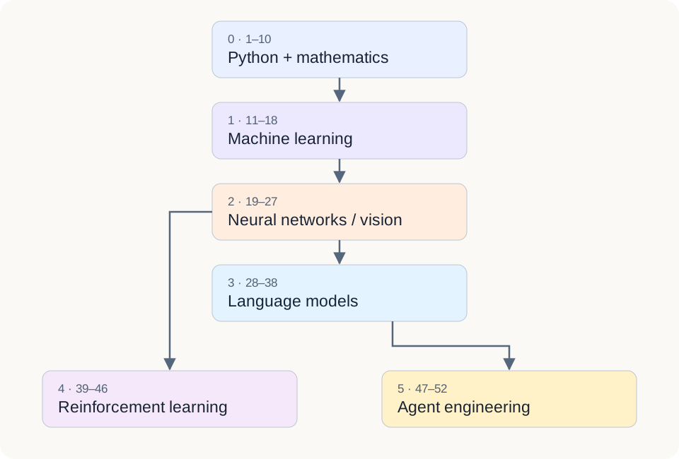
A realistic year and weekly routine
Use one main course per subject. The alternatives solve different needs: visual intuition, slower derivations, additional implementation practice or a specialist branch. Watching three overlapping introductions usually delays the first independent implementation. Keep a resource in reserve until you can name a concrete gap it addresses.
A 12-hour week can allocate 3 hours to lectures and notes, 2 to reconstructing a derivation, 5 to implementation and debugging, and 2 to a short technical report. Pause the video before a derivation or demo and predict the next step. Keep a question log: the mistaken assumption, the smallest counterexample and the changed implementation. Revisit that log after one week and one month.
The schedule is a planning envelope, not a deadline. Weeks 1–10 cover foundations; 11–18 classical ML; 19–27 neural networks; 28–38 language models; 39–46 RL; 47–52 agents. If a project is incomplete, reduce electives before removing implementation time. Do not publicly post solutions to active graded assignments where the course policy forbids it.
Stage 0 · Python and mathematical language
Python is the experimental language: functions express reusable computations, arrays express batches, and tests expose incorrect assumptions. Choose CS50P for self-paced work or Code in Place when a suitable cohort is available. Learn file input, exceptions, virtual environments, Git and reproducible commands. Then learn NumPy broadcasting and PyTorch tensors; the introductory Python course alone does not cover the numerical stack.
For linear algebra, first use 3Blue1Brown to visualize a matrix as a transformation, then work through selected MIT 18.06 topics: linear systems, span, rank, projections, eigenvectors and singular values. ENGR108 is an applied alternative based on the Boyd–Vandenberghe material; its current course uses Julia, so translate the mathematical ideas deliberately rather than expecting Python notebooks. Do not confuse a change in course number with an identical current syllabus.
Probability describes uncertainty over data, while calculus describes sensitivity to parameters. Learn conditional probability, Bayes’ rule, expectation, variance and sampling from CS109 or Stat 110. Use the calculus animations for intuition, then derive partial derivatives and the chain rule on paper. These are not decorative prerequisites: cross-entropy is a probabilistic objective and backpropagation is the chain rule applied to a computation graph.
A small shape example connects the subjects. Let X contain n rows and d features, w contain d weights, and y contain n targets. Xw has n predictions. For mean half-squared error, the gradient is Xᵀ(Xw−y)/n and has d entries. With
Understand the mechanism
A vector is an ordered collection of coordinates; a matrix describes a linear operation between coordinate spaces. Rank tells you how many independent directions survive that operation. If two input features always move together, the data cannot uniquely identify their separate effects without additional assumptions. A derivative measures a local rate of change. A gradient collects partial derivatives, and gradient descent moves opposite that vector because its directional derivative is negative for a sufficiently small step. Probability adds a different idea: uncertainty is represented by a distribution, not by an arbitrary confidence adjective.
A worked decision
Suppose urgent tickets occur with probability 0.01. A detector catches 90% of urgent tickets but flags 5% of nonurgent ones. Among 10,000 tickets, expect 90 true alerts and 495 false alerts: only 90/585≈15.4% of alerts are actually urgent. This is a synthetic Bayes example, not a product measurement. It explains why “90% detection” is insufficient, and why the base rate belongs in both ML evaluation and agent safety discussions.
Suggested weekly sequence
Weeks 1–3: functions, collections, files, exceptions and a reproducible Python environment; use CS50P or a Code in Place cohort. Weeks 4–7: vector operations, matrix products, projections and least squares from selected MIT 18.06 units, with 3Blue1Brown before difficult geometric ideas. Weeks 8–10: conditional probability, expectation and derivatives; connect them to the regression calculation. Study mathematics alongside small programs rather than waiting to finish an entire mathematics curriculum before coding.
X∈ℝⁿˣᵈ, w∈ℝᵈ, y∈ℝⁿ; n>0. The gradient and w have the same shape. This example has no separate bias: the first column of X is constant.
Official resources for this stageStage 1 · Learn from data, not from leakage
Use CS229 as the mathematical spine, with the public 2018 lectures as one stable entry point. The current course homepage can contain restricted material; keep a consistent public edition instead of mixing assignment versions. If the probability notation is overwhelming, use the Andrew Ng specialization as an optional bridge, or Cornell CS4780 as an alternative explanation. Neither replaces doing derivations and implementing a baseline.
Supervised learning estimates a mapping from labeled examples; unsupervised learning looks for structure without target labels. Linear regression predicts a real value, logistic regression estimates a binary probability, and k-means alternates assigning points and updating centroids. Explain the objective before selecting the algorithm. A distance-based method also inherits your feature scaling: a large numerical unit can dominate Euclidean distance.
Use incident-ticket triage as a running scenario: predict whether a ticket requires urgent review from public or synthetic features. Split by time or customer before fitting preprocessing. If near-duplicate tickets cross the split, a strong score can merely measure memorization. Accuracy also hides rare urgent cases; the cost of a missed urgent ticket differs from the cost of an unnecessary review. A model is useful only relative to that decision.
Regularization trades training fit for stability. In ridge regression, λ‖w‖²/2 adds λw to the data gradient. A larger λ is not automatically better: select it using training/validation data and keep the final test partition untouched. Maintain a simple constant or linear baseline before adding model complexity. Save preprocessing, the split manifest and the model together so inference uses the same feature definition.
Understand the mechanism
An estimator maps observed data to parameters; a predictor maps a new input to an output using those parameters. Training loss measures fit on data used for estimation. Generalization concerns unseen data drawn under a stated deployment assumption. Optimization error, estimation error and distribution shift are different problems: more training steps may reduce the first while leaving the others unchanged. Before tuning a model, identify which problem you actually have.
A worked decision
For logistic regression,
Suggested weekly sequence
Weeks 11–13: linear and logistic regression, maximum likelihood and gradients. Weeks 14–16: regularization, validation, feature scaling and k-means. Weeks 17–18: turn one licensed dataset into a documented baseline project. Read relevant CS229 notes after the lecture, derive one objective without the notes, then implement it. Use Cornell only for the topics whose explanations remain unclear; do not restart the whole subject.
λ≥0 controls the penalty; the numerical scale depends on feature normalization and the loss convention.
Official resources for this stageStage 2 · Neural networks and visual representations
Begin Zero to Hero with micrograd: implement scalar computation nodes and accumulate derivatives backwards. Then learn why batched matrix operations are faster than Python loops and why broadcasting can silently create an incorrect gradient. CS231n supplies the next layer: losses, optimization, convolutional features and training practice. Michigan’s vision course is an alternative, not an additional compulsory full course.
A hidden layer learns a representation rather than receiving all useful features by hand. Nonlinearity matters: stacking linear maps still yields one linear map and cannot solve XOR. Backpropagation computes derivatives; Adam or SGD uses those derivatives to update parameters. A low training loss says nothing by itself about generalization. Data augmentation changes the effective training distribution and must preserve the intended label.
A convolution shares a local filter across spatial positions; a vision Transformer relates image patches through attention. These encode different assumptions and compute patterns. For a first vision project, use a small dataset and compare a frozen pretrained feature extractor with fine-tuning under the same data split. A ViT trained from scratch is usually an unnecessarily expensive first experiment. Record the checkpoint license, resolution, trainable parameter count and hardware.
Choose electives after the core. fast.ai is a practical top-down alternative for programmers; MIT 6.S191 is a compact overview; CS230 offers another training-oriented perspective. Generative modeling is a branch: CS236 provides probabilistic modeling, while MIT 6.S184 develops flow matching and diffusion using ODE/SDE ideas. Do not insert every branch into a nine-week main track.
Understand the mechanism
Automatic differentiation applies local derivative rules through a computational graph. When a value feeds two later operations, its gradient is the sum of both paths. This explains why zeroing gradients and accumulating gradients are distinct operations. A training step normally performs forward computation, loss construction, gradient reset, backward computation and optimizer update. Evaluation changes dropout and normalization behavior and disables unnecessary graph recording; it does not merely reuse the training loop without updating weights.
A worked decision
Consider a dense layer with 32 input features and 64 hidden units. It contains 32×64+64=2,112 parameters including bias. A following 10-class layer adds 64×10+10=650, for 2,762 total. Parameter count does not equal training memory: activations, gradients and optimizer state also occupy memory. Adam typically maintains two moment tensors per trained parameter; the exact byte budget depends on dtype, master weights and implementation. Start by accounting for tensors before renting a larger GPU.
Suggested weekly sequence
Weeks 19–21: micrograd, chain-rule accumulation and small multilayer networks. Weeks 22–24: vectorized training, initialization, optimizer behavior and convolutional representations. Weeks 25–27: selected vision assignments and one frozen-versus-fine-tuned comparison. Keep generative modeling elective. If a training run fails, reason about its data and gradient flow before replacing the architecture.
For X:[n,d], W₁:[d,h], b₁:[h], W₂:[h,c] and b₂:[c], hidden states are [n,h] and predictions [n,c]. σ is an elementwise nonlinearity; bias broadcasts over rows.
Official resources for this stageStage 3 · From text to a trained language model
CS224N connects language tasks, embeddings, sequence models and attention. Follow the official public 2024 recordings and inspect the matching materials; current enrolled-student recordings are a separate access tier. An embedding maps a token ID to a learned vector. It is not a database fact: proximity can encode statistical association without truth, authorization or provenance.
A tokenizer maps bytes or text into discrete IDs. BPE learns repeated-symbol merges; changing the tokenizer changes sequence lengths, vocabulary size and the model’s prediction problem. A decoder-only Transformer predicts the next token under a causal mask. For Q and K with shape [T,dₖ], QKᵀ has shape [T,T]; multiplying normalized attention by V of shape [T,dᵥ] returns [T,dᵥ]. The mask prevents position t from reading later positions during training.
Cross-entropy averages negative log probability assigned to the correct next token. If the correct-token probability is 0.25, that token contributes about 1.386 nats. Compare validation losses only under compatible tokenization, data and loss aggregation. A low next-token loss does not certify factuality or safe tool use. Padding masks, shifted labels and data contamination are engineering details with mathematical consequences.
Use CS336 assignment 1 as the main implementation target: a tokenizer, decoder model, optimizer and training loop on a deliberately small corpus. CS336 as a whole expects strong Python/PyTorch and systems knowledge; its full workload does not fit into this stage for every beginner. Start on a tiny subset, save configuration and checkpoints, then expand only after correctness is established. Token count, context length and batch size determine both memory and training budget.
CME295 is an architectural overview; its official syllabus now separates 2025 and 2026. Hugging Face adds ecosystem practice. CS25 is a research seminar, not a substitute for a sequential implementation course. CMU advanced NLP is useful when a specific research question emerges. Keep pretraining, supervised fine-tuning, retrieval augmentation and inference separate: they change weights, context or execution in different ways.
Understand the mechanism
A next-token dataset is a shifted sequence pair. From IDs [4,7,9,2], an input [4,7,9] has targets [7,9,2]. With batch B, sequence T and vocabulary V, logits have shape [B,T,V]. Cross-entropy selects the target entry at each unmasked position and reduces over valid positions. Merely reshaping a tensor can keep every dimension legal while shifting labels incorrectly. Separately, BPE training chooses token merges; Transformer training learns parameters conditional on the resulting token IDs.
A worked decision
A tiny reference configuration might use
Suggested weekly sequence
Weeks 28–30: language tasks, embeddings and causal attention using selected CS224N material. Weeks 31–33: byte handling and BPE, then one decoder block. Weeks 34–36: the complete small-model training loop, checkpoint and generation path from CS336 assignment 1. Weeks 37–38: interpret held-out behavior and write a model/data card. After this, choose systems profiling, multilingual data, RAG or post-training rather than trying to train a commercially competitive model.
Softmax is row-wise;
Stage 4 · Learning through decisions and rewards
Reinforcement learning chooses actions whose effects unfold over time. In a Markov decision process, state summarizes information needed for the next transition, action changes the environment, reward supplies a scalar objective, and γ discounts later rewards. If a task is simply predicting fixed labels, supervised learning is usually a simpler starting point. An LLM calling a tool is not automatically doing RL.
Use CS234 for values, Bellman equations and policy evaluation, with Sutton–Barto or David Silver as supporting explanations. Then select CS285 material on function approximation, policy gradients and actor–critic learning. DQN approximates action values for discrete actions and stabilizes updates with replay and target networks. PPO updates a policy using a clipped surrogate objective; clipping is a practical restriction on updates, not a universal safety guarantee.
The one-step target r+γ maxₐ Q(s′,a) bootstraps from a future estimate. With
Treat LLM post-training as an advanced branch after toy-environment competence. CS224R and CS329H connect policies and preferences; the latter has official 2026 course materials but this guide does not promise public videos. GRPO is not a cheap shortcut to reasoning: reward validity, sampled groups, KL control and held-out tasks matter, and gains can reflect reward exploitation. Old Spinning Up code is valuable for algorithms but may require dependency adaptation rather than running unchanged with modern Gymnasium.
Understand the mechanism
A policy specifies how actions are selected; a value function estimates future return. The environment, not the learner, produces the next observation and reward. On-policy methods learn from data generated by the policy they are updating; off-policy methods can reuse other behavior, but must manage the resulting mismatch. Replay is therefore part of an algorithm’s assumptions rather than a universally safe speedup. Partial observations can also invalidate the assumption that the current observation is a sufficient state.
A worked decision
With rewards [1,0,2] and
Suggested weekly sequence
Weeks 39–41: MDPs, Bellman updates and tabular reasoning through CS234. Weeks 42–44: function approximation, DQN and policy gradients with selected CS285 units. Weeks 45–46: a scoped DQN/PPO comparison and a failure analysis. The advanced LLM-RL branch comes later: first understand where rewards originate, what data policy produced a trajectory and how much environment interaction was used.
Stage 5 · Build a bounded, observable agent
An agent is a system that repeatedly selects actions using observations and a task objective. A deterministic workflow fixes the sequence in advance; an agent lets a model select some steps. Start with the smallest useful autonomy. For ticket triage, a first system can retrieve public runbooks, cite evidence and propose a diagnostic command without executing a production change.
CS329Z supplies the implementation spine: core components before framework abstractions. Its current public schedule has video links for the first five sessions as checked on November 14, 2026; do not assume the whole quarter is already available. The two homework assignments cover harness construction and evaluation design. Follow the official repository instructions and costs rather than copying a social-media claim about a fixed total API bill.
Use Berkeley’s Fall 2024 series to establish the agent landscape, Spring 2025 for advanced reasoning and verifiable tasks, and Fall 2025 Agentic AI for additional system perspectives. These are archived lecture series; old certificate deadlines are not current enrollment offers. Watch selected talks after identifying a gap in your project. Hugging Face provides another practical path; CS329A and CS222 are research/readings branches.
A minimal harness owns a message ledger, tool schemas, parsing, authorization, execution, result normalization and a stop rule. The model proposes an action; trusted code checks the tool name, arguments and current permission. Tool output is untrusted data, not a new system instruction. Persist state before irreversible work, define idempotency and timeout behavior, and ask for human approval where the action risk requires it. A prompt saying “be careful” does not create an enforcement boundary.
Set explicit step, time and token limits. If each of eight calls uses at most 2,000 input tokens and 300 output tokens, the upper budget is 18,400 tokens, excluding separately budgeted retries and auxiliary calls. A local stub can exercise the control flow without a paid model. An end-to-end agent also needs task-level evidence: tool correctness alone does not prove that the user’s objective was achieved.
Understand the mechanism
Separate three interfaces: the model adapter translates messages into model requests; the harness governs state and decisions; the tool executor implements approved effects. Store typed events such as model_proposal, tool_denied, tool_started and tool_result. A state machine might move ready→proposed→authorized→executing→observed, with explicit denied, timed_out and stopped outcomes. An exception must not silently become a successful observation. A durable event log supports investigation, but replaying a log is not permission to repeat a side effect.
A worked decision
For an incident assistant, start with three read-only tools: search_runbooks(query), get_service_metrics(service,window) and fetch_recent_changes(service). Model-provided service names must be checked against the user’s allowed scope. The response should distinguish observed metrics, retrieved recommendations and model inference. If metrics time out, return an incomplete-evidence result rather than inventing healthy values. Adding restart_service changes the risk class and needs a separate authorization/approval design; it is not just another function schema.
Suggested weekly sequence
Weeks 47–48: implement a deterministic retrieval-and-answer workflow and a fake model adapter. Weeks 49–50: allow bounded tool selection, persist state and define refusal/timeout behavior; follow the relevant CS329Z harness components. Weeks 51–52: design a held-out task set, analyze traces and assemble a reproducible final demonstration. Use Berkeley talks to answer emerging design questions. Six weeks is a scoped learning project, not a promise to complete every official assignment at full course scope.
A synthetic upper bound for model input/output tokens. Each call must satisfy its own cap; retries, judges and embeddings are not included.
Official resources for this stageChoose a specialization without restarting
For an AI application engineer, emphasize stage 3 inference and stage 5 reliability, plus retrieval, security and observability. For an ML researcher, invest more time in probability, optimization, derivations and controlled experiments. For robotics, extend RL with estimation, control, dynamics and simulation-to-real transfer; the six-stage route alone is not a robotics qualification.
A coherent portfolio can contain a classical baseline, a vision model, a tiny language model, an RL learning report and a bounded agent. Keep the connecting story: what data enters, what is learned, what executes, what is measured and what remains unknown. Completing courses cannot guarantee expertise or employment; the evidence below is a more honest measure than a playlist completion percentage.
Practice, projects and evidence of mastery
All hands-on verification is collected here after the conceptual route. The examples are original teaching exercises, not official course solutions. Pin a course edition and follow its honor code. External assignments run in your own environment; do not upload private tickets or credentials.
Foundations
Practice evidence. Create a CSV-to-feature pipeline and reproduce the two-row regression example. Include a clean-environment command, shape assertions and a finite-difference gradient check.
Failure / fair comparison. Failure case: shuffle target rows without features. Explain why a valid shape does not imply a valid dataset.
Build it in this order
- Create a repository with src/, tests/, data/ and a README; use a virtual environment and record Python/package versions. Load a tiny CSV, preserve row identifiers and implement the numerical examples before introducing a library estimator.
- Save one command that recreates outputs from a fresh checkout. Then alter one input, predict the change on paper and verify it. If the prediction fails, explain the discrepancy rather than only changing the code until the test passes.
Classical ML
Practice evidence. Implement linear/logistic regression and k-means with NumPy. On one licensed public dataset, report a constant baseline, time/group-aware split, preprocessing fitted only on training data and a final untouched test result.
Failure / fair comparison. Compare two regularization settings under the same split. Inspect rare-class recall and leakage rather than selecting the best test result.
Build it in this order
- Define the decision, labels and split manifest before exploring validation scores. Implement preprocessing fit/transform separately, then constant, linear/logistic and clustering baselines. K-means does not require class labels for training.
- Keep train/validation/test roles fixed. Record each experiment’s parameters and result, select once using validation, then evaluate the final model on test. Include at least one failure slice such as a rare group or later time period.
Deep learning
Practice evidence. Complete selected CS231n or Michigan assignments, then compare a frozen encoder with fine-tuning on one small vision task. Record seed, checkpoint, transformations, learning rate and hardware.
Failure / fair comparison. First overfit a tiny training subset to debug the pipeline. Inspect mislabeled data and keep validation transforms deterministic.
Build it in this order
- Build a data loader, model, loss, optimizer and training function as separate components. Log learning rate, training/validation loss and gradient norms; save a small known-input batch for debugging.
- First train a small network, then reuse one licensed pretrained checkpoint. Compare frozen features with fine-tuning under the same split and comparable resource constraints. Explain any advantage that comes from extra pretrained data rather than from your own method.
Language modeling
Practice evidence. Complete the scoped CS336 assignment-1 path. Save tokenizer rules, model configuration, data hashes, optimizer state and a small sampling command. Link a loss curve and explain each tensor shape.
Failure / fair comparison. Test tokenizer round trips, causal invariance and checkpoint reload. Compare learned predictions with a unigram baseline on a held-out corpus; do not compare incompatible tokenizers by perplexity alone.
Build it in this order
- Build tokenizer encode/decode; construct shifted input/target pairs; implement embeddings, causal attention, feed-forward blocks and output projection; add loss, optimizer and a sampling entry point.
- Checkpoint model, optimizer, scheduler, step number, configuration and RNG state when exact continuation matters. Resume a short run and compare with uninterrupted training under deterministic settings. Store data hashes and report remaining nondeterminism.
Reinforcement learning
Practice evidence. Implement DQN and PPO on small Gymnasium tasks. Report multiple seeds, environment/version, total interaction steps, evaluation policy and distributions rather than only the best run.
Failure / fair comparison. Check terminal versus truncated handling. Compare at equal interaction budgets; if compute differs, report it. A failed run and its diagnosis belong in the report.
Build it in this order
- Use one small discrete-action environment for DQN and an appropriately configured task for PPO. Keep environment wrappers, episode limits and preprocessing explicit. Distinguish training exploration from evaluation action selection.
- Choose seeds and budgets before running. Store learning curves against environment steps and wall-clock separately. Diagnose at least one deliberate reward or terminal-handling error, then restore the correct implementation and document the difference.
Agent system
Practice evidence. Work through CS329Z HW1/HW2 at the official scope. Build a read-only local incident assistant with a scripted-model baseline, trace IDs, tool allowlist, state persistence and explicit stop conditions.
Failure / fair comparison. Inject malformed tool output, prompt injection, timeout and duplicate delivery. Separate deterministic control-flow tests from model-quality tests. Use held-out tasks; do not trust an uncalibrated model judge as ground truth.
Build it in this order
- Implement the model adapter and three read-only tools; add schema validation, current-scope authorization, step/token limits, trace IDs and persistent events. Run a scripted model first so failures are reproducible.
- Introduce a real local model only after control checks pass. Evaluate task outcome, evidence support, denied actions, latency and resource use separately. Package the repository, environment instructions, example traces and limitations; never put credentials in it.
This downloadable Python 3.11+ foundation check uses only the standard library, no network, random numbers or API key. It reproduces the numerical examples and checks a gradient using central differences. It is a small entry exercise, not an implementation of all six capstones. The later projects use their official repositories and Token Lab’s from-zero tutorials.
Download codepython3 roadmap-foundations.py"""Python 3.11+, standard library only; deterministic synthetic examples."""
import math
X = [[1.0, 0.0], [1.0, 1.0]]
y = [1.0, 3.0]
w = [0.0, 0.0]
def loss(weights):
errors = [sum(a * b for a, b in zip(row, weights)) - target
for row, target in zip(X, y)]
return sum(e * e for e in errors) / (2 * len(y))
def gradient(weights):
errors = [sum(a * b for a, b in zip(row, weights)) - target
for row, target in zip(X, y)]
return [sum(row[j] * e for row, e in zip(X, errors)) / len(y)
for j in range(len(weights))]
def softmax(logits):
if not logits or not all(math.isfinite(v) for v in logits):
raise ValueError("finite, nonempty logits required")
maximum = max(logits)
values = [math.exp(v - maximum) for v in logits]
return [v / sum(values) for v in values]
def td_target(reward, gamma, next_values, terminated):
return reward if terminated else reward + gamma * max(next_values)
g = gradient(w)
eps = 1e-6
for j, analytic in enumerate(g):
plus, minus = w.copy(), w.copy()
plus[j] += eps
minus[j] -= eps
numeric = (loss(plus) - loss(minus)) / (2 * eps)
assert math.isclose(analytic, numeric, abs_tol=1e-8)
updated = [a - 0.1 * b for a, b in zip(w, g)]
assert loss(updated) < loss(w)
p = softmax([1000.0, 1000.0])
assert p == [0.5, 0.5]
assert math.isclose(sum(softmax([1.0, 2.0, 3.0])), 1.0)
try:
softmax([])
except ValueError:
pass
else:
raise AssertionError("empty inputs must fail")
assert td_target(1, 0.9, [2, 4], True) == 1
assert math.isclose(td_target(1, 0.9, [2, 4], False), 4.6)
print(f"gradient={g}")
print(f"weights={[round(v, 2) for v in updated]}")
print(f"loss={loss(updated):.6f}")
print(f"cross_entropy={-math.log(0.25):.6f}")
print(f"td_target={td_target(1, 0.9, [2, 4], False):.1f}")
# Additional synthetic decision/resource examples in the expanded tutorial.
base_rate, sensitivity, false_positive_rate = 0.01, 0.90, 0.05
true_alerts = 10_000 * base_rate * sensitivity
false_alerts = 10_000 * (1 - base_rate) * false_positive_rate
precision = true_alerts / (true_alerts + false_alerts)
assert true_alerts == 90 and false_alerts == 495
assert math.isclose(precision, 90 / 585)
miss_cost, false_alert_cost = 20, 1
threshold = false_alert_cost / (miss_cost + false_alert_cost)
assert math.isclose(threshold, 1 / 21)
for probability in (0.01, 0.05, 0.9):
flag = probability > threshold
assert flag == ((1 - probability) * false_alert_cost < probability * miss_cost)
assert 32 * 64 + 64 + 64 * 10 + 10 == 2762
assert 4 * 128 * 1024 * 4 == 2 * 1024**2
assert math.ceil(100_000 / (4 * 128)) == 196
assert math.isclose(sum(0.9**i * reward for i, reward in enumerate([1, 0, 2])), 2.62)
print("checks=passed")
Expected output:
Original interview questions and scoring
Why is a high test score not sufficient evidence of learning?
Hint
Check how examples and preprocessing crossed the split.
Answer and analysis
Duplicate or future information can leak; repeated test-set tuning also invalidates a held-out claim. Rebuild a group/time-aware split, fit transforms on training data and compare a baseline with uncertainty.
Why can training all Transformer positions at once still be autoregressive?
Hint
Separate parallel arithmetic from permitted information flow.
Answer and analysis
A causal mask prevents future-token attention. Labels are shifted by one position. Changing a future input must not change earlier outputs in evaluation mode, up to numerical tolerance.
Must an agent use reinforcement learning?
Hint
Distinguish selecting actions at inference from updating a policy.
Answer and analysis
No. A pretrained model with a bounded harness can select tools without online weight updates. RL is one way to improve a policy; it adds reward-design and evaluation requirements.
When should a learner add a framework?
Hint
First name the repeated mechanism the framework replaces.
Answer and analysis
After implementing and understanding state transitions, parsing, tool execution and failures. A framework can reduce boilerplate, but its defaults do not prove authorization, durable execution or task success.
Use this 1–5 rubric for every project: 1 = repeat terminology; 2 = explain the mechanism and assumptions; 3 = independently reproduce the baseline and numerical checks; 4 = diagnose failures and compare a matched-budget alternative; 5 = defend design choices, uncertainty, limitations and a transfer experiment. Require at least 3 on correctness, reproducibility and explanation before advancing; a polished demo cannot compensate for missing evidence.
What to do when you get stuck
If a formula is unclear, reduce it to one scalar or a two-row matrix and compute every intermediate value. If code is unclear, isolate one function and inspect inputs, shapes and state. If training is unclear, compare with the simplest baseline and a tiny dataset. If a paper is unclear, separate its claim, assumptions, evidence and limitations.
Use an AI assistant as a tutor: ask for a hint, a counterexample or a critique of your derivation before requesting a complete solution. Close the generated answer and reconstruct the implementation yourself. Keep a short explanation of every borrowed component, including its license and tests; a passing generated solution is not evidence that you can maintain it.
Predict, test and keep evidence
Before revealing an answer, predict one result. After the exercise, record the discrepancy and a transfer test. Saved locally across language editions.
Open notebook / export / clear →The mathematical review scope is recorded per lesson. It does not establish empirical paper reproduction; report suspected errors in your notes. Review scope
Official courses, videos and further study
Links point to original providers. The catalogue is a verified starting map, not a guarantee that every current lecture, exercise, certificate or compute resource is free. Use the provider’s syllabus for its video links when a stable direct playlist was not verified. Course editions, public recordings and assignment dependencies can differ. Verification date: November 14, 2026.
Stage 0 · Python and mathematical language
CS50Phttps://cs50.harvard.edu/python/
Core selection; use the syllabus for lectures and assignments.
Stanford Code in Placehttps://codeinplace.stanford.edu/
Cohort-based; check application dates. CS50P is the self-paced alternative.
3Blue1Brown · Linear algebrahttps://www.3blue1brown.com/topics/linear-algebra
Visual intuition before formal derivation; not a university course or a replacement for exercises.
Course / materialshttps://www.3blue1brown.com/topics/linear-algebra
MIT 18.06 · Gilbert Strang · 2010https://ocw.mit.edu/courses/18-06-linear-algebra-spring-2010/
Core selection; use the syllabus for lectures and assignments.
Course / materialshttps://ocw.mit.edu/courses/18-06-linear-algebra-spring-2010/ · Video / companion materialhttps://ocw.mit.edu/courses/18-06-linear-algebra-spring-2010/video_galleries/video-lectures/
Stanford ENGR108https://web.stanford.edu/class/engr108/
Applied linear algebra; current course uses Julia.
Stanford CS109https://web.stanford.edu/class/cs109/
Probability for programming; reader linked. Current recordings can require enrollment.
Course / materialshttps://web.stanford.edu/class/cs109/ · Video / companion materialhttps://probabilitycoders.stanford.edu/
Harvard Stat 110https://stat110.hsites.harvard.edu/
Alternative explanation or course; do not add another full overlapping course by default.
3Blue1Brown · Calculushttps://www.3blue1brown.com/topics/calculus
Visual intuition before formal derivation; not a university course or a replacement for exercises.
Course / materialshttps://www.3blue1brown.com/topics/calculus
Stage 1 · Learn from data, not from leakage
Stanford CS229 · 2018 lectureshttps://cs229.stanford.edu/
Public 2018 lecture entry; some current materials are restricted.
Course / materialshttps://cs229.stanford.edu/ · Video / companion materialhttps://www.youtube.com/watch?v=jGwO_UgTS7I
Machine Learning Specialization · Andrew Nghttps://www.coursera.org/specializations/machine-learning-introduction
Optional bridge; do not assume all access or certificates are free.
Course / materialshttps://www.coursera.org/specializations/machine-learning-introduction
Cornell CS4780 · 2018https://www.cs.cornell.edu/courses/cs4780/2018fa/
Alternative explanation or course; do not add another full overlapping course by default.
Course / materialshttps://www.cs.cornell.edu/courses/cs4780/2018fa/ · Video / companion materialhttps://www.youtube.com/playlist?list=PLl8OlHZGYOQ7bkVbuRthEsaLr7bONzbXS
Stage 2 · Neural networks and visual representations
Karpathy · Neural Networks: Zero to Herohttps://karpathy.ai/zero-to-hero.html
Core selection; use the syllabus for lectures and assignments.
Stanford CS231nhttps://cs231n.stanford.edu/
Official public playlist linked; Spring 2026 recordings are enrolled-student access.
Course / materialshttps://cs231n.stanford.edu/ · Video / companion materialhttps://www.youtube.com/playlist?list=PLoROMvodv4rOmsNzYBMe0gJY2XS8AQg16
UMich EECS498/598 · 2019 assignment archivehttps://web.eecs.umich.edu/~justincj/teaching/eecs498/FA2019/assignment2.html
2019 assignment archive is accessible; the old homepage returned 404 during checking. Use as an assignment alternative, not a verified complete-video package.
Course / materialshttps://web.eecs.umich.edu/~justincj/teaching/eecs498/FA2019/assignment2.html
3Blue1Brown · Neural networkshttps://www.3blue1brown.com/topics/neural-networks
Visual intuition before formal derivation; not a university course or a replacement for exercises.
Course / materialshttps://www.3blue1brown.com/topics/neural-networks
fast.ai · Practical Deep Learninghttps://course.fast.ai/
Alternative explanation or course; do not add another full overlapping course by default.
MIT 6.S191https://introtodeeplearning.com/
Optional overview; use official lesson links and distinguish current from archived editions.
Stanford CS230https://cs230.stanford.edu/
Specialist supplement after the core; select topics that address a concrete gap.
Stanford CS236 · Deep Generative Modelshttps://deepgenerativemodels.github.io/
Generative-model branch; probability and calculus first. Companion link may be lecture-note PDF rather than video.
MIT 6.S184 · 2026https://diffusion.csail.mit.edu/2026/index.html
Generative-model branch; probability and calculus first. Companion link may be lecture-note PDF rather than video.
Course / materialshttps://diffusion.csail.mit.edu/2026/index.html · Video / companion materialhttps://diffusion.csail.mit.edu/2026/docs/lecture_notes.pdf
Stage 3 · From text to a trained language model
Stanford CS224Nhttps://web.stanford.edu/class/cs224n/
Public 2024 playlist; current course recordings and public materials have different access.
Course / materialshttps://web.stanford.edu/class/cs224n/ · Video / companion materialhttps://www.youtube.com/playlist?list=PLoROMvodv4rOaMFbaqxPDoLWjDaRAdP9D
Stanford CS336 · Spring 2026https://cs336.stanford.edu/
2026 videos and assignments; strong implementation prerequisites. Scope year one to assignment 1 before optional systems work.
Course / materialshttps://cs336.stanford.edu/ · Video / companion materialhttps://www.youtube.com/playlist?list=PLoROMvodv4rMqXOcazWaTUHhq-yembLCV
Stanford CME295https://cme295.stanford.edu/syllabus/
Optional overview; use official lesson links and distinguish current from archived editions.
Stanford CS25https://web.stanford.edu/class/cs25/
Research seminar: follow selected talks after foundational implementation.
CMU 11-711 · Advanced NLP · 2024https://phontron.com/class/anlp2024/
Specialist supplement after the core; select topics that address a concrete gap.
Hugging Face LLM Coursehttps://huggingface.co/learn/llm-course/
Practical ecosystem course; dependencies and external compute are separate requirements.
Stage 4 · Learning through decisions and rewards
Sutton & Barto · Reinforcement Learning, second editionhttp://incompleteideas.net/book/the-book-2nd.html
Free author-hosted textbook; fetch was unavailable during this check, so availability is not certified here.
Course / materialshttp://incompleteideas.net/book/the-book-2nd.html
David Silver · RL · 2015https://davidstarsilver.wordpress.com/teaching/
Alternative explanation or course; do not add another full overlapping course by default.
Course / materialshttps://davidstarsilver.wordpress.com/teaching/
Stanford CS234https://web.stanford.edu/class/cs234/
Core selection; use the syllabus for lectures and assignments.
Berkeley CS285 · 2023 lectureshttps://rail.eecs.berkeley.edu/deeprlcourse/
Official 2023 playlist; choose matching archived assignments rather than mixing editions.
Course / materialshttps://rail.eecs.berkeley.edu/deeprlcourse/ · Video / companion materialhttps://www.youtube.com/playlist?list=PL_iWQOsE6TfVYGEGiAOMaOzzv41Jfm_Ps
Stanford CS224Rhttps://cs224r.stanford.edu/
Specialist supplement after the core; select topics that address a concrete gap.
OpenAI Spinning Uphttps://spinningup.openai.com/en/latest/
Algorithm explanations and older implementations; check dependency compatibility.
Hugging Face Deep RL Coursehttps://huggingface.co/learn/deep-rl-course/en/unit0/introduction
Practical ecosystem course; dependencies and external compute are separate requirements.
Course / materialshttps://huggingface.co/learn/deep-rl-course/en/unit0/introduction
Stanford CS329H · Autumn 2026https://web.stanford.edu/class/cs329h/
2026 preference-learning materials; public lecture video availability not verified.
Stanford CS221https://stanford-cs221.github.io/autumn2025/
Select MDP/game topics. The 2025 page lists Canvas recordings and public slides/code.
Course / materialshttps://stanford-cs221.github.io/autumn2025/
Stage 5 · Build a bounded, observable agent
Stanford CS329Z · Autumn 2026https://cs329z.stanford.edu/
2026 course; five public lecture links checked, more may be released. HW1 builds a harness; HW2 designs an evaluation task.
Course / materialshttps://cs329z.stanford.edu/ · Video / companion materialhttps://youtu.be/DGI4vucR71w
Berkeley LLM Agents · Fall 2024https://llmagents-learning.org/f24
First Berkeley series: agent foundations. Archived certificate dates are not current offers.
Berkeley Advanced LLM Agents · Spring 2025https://llmagents-learning.org/sp25
Second series: advanced reasoning and verifiable tasks.
Berkeley Agentic AI · Fall 2025https://agenticai-learning.org/f25
Third series: Agentic AI. Select talks after the first series rather than treating all three as prerequisites.
Stanford CS329A · Self-Improving AI Agentshttps://cs329a.stanford.edu/
Research branch on self-improving agents; requires evaluation and failure analysis.
Stanford CS222 · Fall 2024https://joonspk-research.github.io/cs222-fall24/
2024 readings/project materials; no verified public full lecture-video series.
Course / materialshttps://joonspk-research.github.io/cs222-fall24/
Hugging Face Agents Coursehttps://huggingface.co/learn/agents-course/en/unit0/introduction
Practical ecosystem course; dependencies and external compute are separate requirements.
Course / materialshttps://huggingface.co/learn/agents-course/en/unit0/introduction
- CS336 · Assignment 1https://github.com/stanford-cs336/assignment1-basics
- CS329Z · HW1https://github.com/cs329z/assignment1-harness
- CS329Z · HW2https://github.com/cs329z/assignment2-evals